

The Ljung–Box Test for Time-Series Autocorrelation
Learn how the Ljung–Box Q statistic combines residual autocorrelations, how to choose lags and degrees of freedom, and what the test cannot establish about financial returns.
In this guideWhat the Ljung–Box test evaluates
Short summary
The Ljung–Box test asks whether autocorrelations through a chosen lag are jointly consistent with zero. Applied to model residuals, it checks for leftover linear dependence over that range; it does not prove independence, normality, model correctness, or a tradable return forecast.
What the Ljung–Box test evaluates
A sample autocorrelation plot can show dependence at several lags, but reading many individual bars creates a multiple-testing problem. The Ljung–Box test combines the first \(h\) sample autocorrelations into one portmanteau statistic. Its null is that the population autocorrelations at lags 1 through \(h\) are all zero. The alternative is that at least one of those correlations differs from zero.
Box and Pierce developed an overall lack-of-fit test for fitted time-series models. Ljung and Box modified its statistic to improve the approximation in finite samples. “Portmanteau” means that one statistic summarizes several lag-specific correlations; it does not mean every kind of time-series dependence has been tested.
For a return series, the question might be whether past signed returns leave linear serial dependence. For a fitted ARMA model, the question is usually whether residual autocorrelation remains after the model has used its specified lag structure. Those are related but distinct applications, so identify the series being tested before interpreting the result.
Calculate the Box–Pierce and Ljung–Box statistics
Let \(\hat\rho_k\) be the sample autocorrelation at lag \(k\), \(n\) the number of observations used to calculate it, and \(h\) the largest lag in the test. The Box–Pierce statistic is
\[ Q_{BP}=n\sum_{k=1}^{h}\hat\rho_k^2. \]
The Ljung–Box adjustment weights each lag by the available sample size:
\[ Q_{LB}=n(n+2)\sum_{k=1}^{h}\frac{\hat\rho_k^2}{n-k}. \]
The squared correlations mean that positive and negative autocorrelation both raise the statistic. The adjustment gives more weight to a given estimated correlation at a lag with fewer usable pairs. In large samples, the two statistics often become close; in finite samples, Ljung–Box is commonly used because its small-sample approximation performed better in the original study.
Under a white-noise null and the test's regularity conditions, \(Q_{LB}\) is compared with a chi-square distribution. For a raw series with no fitted dynamic parameters, the reference degrees of freedom are commonly \(h\). For residuals from an estimated ARMA(\(p,q\)) model, the common adjustment is \(h-p-q\), provided it is positive. The correction reflects parameters used to fit the residual dynamics; it is not a universal instruction to subtract every coefficient in any regression. Integrated, seasonal, constrained, or otherwise specialized models can require different conventions. Match the reference degrees of freedom to the exact residual test and software definition. For example, testing ARMA(2,2) residuals only through \(h=4\) leaves zero degrees of freedom under the common adjustment. The ordinary chi-square comparison is unavailable; choose a longer prespecified lag range or a diagnostic designed for that model rather than forcing a zero-degree reference. Report why the lag horizon was chosen.
Work through a hypothetical residual calculation
Suppose a fitted model leaves \(n=250\) residuals, and a prespecified five-lag check produces autocorrelations \(0.10, 0.05, -0.08, 0.02, -0.04\). The Box–Pierce calculation first squares and sums them:
\[ 0.10^2+0.05^2+(-0.08)^2+0.02^2+(-0.04)^2=0.0209. \]
Then \(Q_{BP}=250(0.0209)=5.225\). Applying the Ljung–Box weights gives
\[ Q_{LB}=250(252)\left(\frac{0.0100}{249}+\frac{0.0025}{248}+\frac{0.0064}{247}+\frac{0.0004}{246}+\frac{0.0016}{245}\right)\approx 5.31. \]
The calculation is not yet a p-value. If these are residuals from an ARMA(1,1) fit, the common reference uses \(h-p-q=5-1-1=3\) degrees of freedom; for a raw series under its own null, it may use five. The degrees-of-freedom choice changes the upper-tail probability. All numbers here are invented to show the arithmetic, not observed market data or a model result.
A small statistic means the observed squared autocorrelations are not unusually large under the selected reference distribution. It does not prove the correlations are exactly zero. A large statistic says the set is difficult to reconcile with the null at the chosen level; inspect which lags and what model features are responsible rather than treating the single number as a diagnosis.
Choose the lag horizon before looking at the most favorable result
The lag limit \(h\) defines the question. Testing only a few short lags can miss slower dependence or a weekly pattern in daily observations. Extending the test to many lags can add weak, noisy estimates, reduce power against a specific short-lag pattern, and make the result sensitive to a few long-lag correlations. A large \(h\) also leaves fewer degrees of freedom after an ARMA adjustment.
Choose lags based on sampling frequency, known calendar structure, model purpose, and the dependence the residuals should no longer contain. For daily market data, a trading-session lag is not always the same as a calendar-day lag. Intraday data may have time-of-day and overnight effects. A seasonal model may call for seasonal lags or a seasonal diagnostic; a single generic cutoff can hide that structure.
If many values of \(h\), transformations, assets, or model orders are tried and only the smallest p-value is reported, the displayed significance ignores that search. State the lag range and decision rule before interpreting the diagnostic, or account for the broader search in the inference plan.
Read the autocorrelation plot with the joint statistic
An autocorrelation plot often includes approximate single-lag bands such as \(\pm1.96/\sqrt{n}\). Under a simple white-noise model, those can help flag an individual sample correlation, but they are not a simultaneous 95% band for every lag. Looking at many bars separately raises the chance that at least one crosses by chance. The Ljung–Box test instead asks one joint question for the prespecified set, using a reference distribution for the combined statistic.
The joint statistic can be raised by one relatively large autocorrelation or by several modest correlations. Inspect the lag-by-lag terms \(n(n+2)\hat\rho_k^2/(n-k)\) and the ACF plot after the test. A single bar outside a heuristic band does not automatically equal a significant portmanteau result, and all bars inside their separate bands do not guarantee that the joint statistic is insignificant.
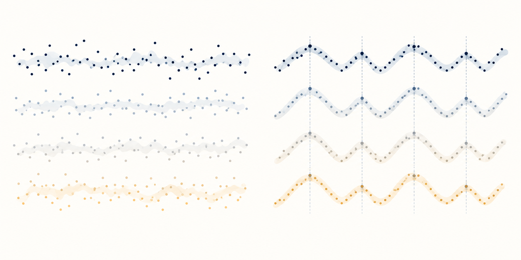
Distinguish raw returns, model residuals, and squared residuals
Applying the test to signed returns asks whether their linear autocorrelation through lag \(h\) is jointly zero. Applying it to fitted residuals asks whether the selected model has left similar linear dependence. A rejection can motivate checking the mean specification, timing, market calendar, and residual plots; it does not identify which term is missing.
Check whether overlapping return windows create dependence
The observation definition can create autocorrelation even when the underlying one-period returns are uncorrelated. For example, a five-session rolling return and the next five-session rolling return share four daily returns. Their overlap mechanically links adjacent observations. Ljung–Box can correctly reject zero autocorrelation in that constructed series without showing that a non-overlapping daily return was forecastable.
State whether observations are daily returns, rolling multi-day returns, or residuals from a model of overlapping outcomes. Align the session calendar, close timestamps, and overnight interval with the economic question. If overlapping horizons are required, use inference and a reference distribution appropriate to that construction rather than interpreting the result as evidence of a standalone trading edge.
Volatility clustering can exist even when signed returns have little autocorrelation. Squaring residuals changes the question: autocorrelation in squared or absolute standardized residuals can indicate dependence in the scale of returns. McLeod and Li study squared-residual autocorrelations as a diagnostic for nonlinear dependence after ARMA fitting. This remains a diagnostic, not proof of one unique volatility model. The ARCH-LM guide covers a more targeted test for ARCH-type dependence, and the GARCH guide explains conditional-variance modeling.
Zero autocorrelation is weaker than independence. A sequence can have zero correlations at the tested lags and still depend on nonlinear transformations, conditional variance, tails, or regimes. The Ljung–Box statistic also says nothing by itself about normality, stationarity, causal structure, or whether a return can be earned after execution costs.
Check the reference distribution when parameters were estimated
The simple chi-square approximation relies on the model, residual construction, sample size, and parameter-estimation setup. If an ARMA model is fitted first, the residual autocorrelations are estimated quantities rather than correlations of directly observed innovations. The usual degrees-of-freedom adjustment is a practical asymptotic convention, not an exact finite-sample guarantee for every specification.
Small samples, a large lag horizon, near-canceling AR and MA roots, outliers, conditional heteroskedasticity, or serial dependence outside the fitted family can make the approximation less reliable. A rejection may reflect a misspecified mean, a data-quality issue, or an unsuitable reference distribution. A non-rejection may reflect low power or a lag choice that omitted the dependence of interest.
For a complex or nonstandard model, use a diagnostic procedure whose reference distribution matches the fit, or assess calibration with a justified bootstrap that repeats the estimation step. Resampling iid residuals is not automatically valid when dependence or changing variance is part of the concern. Explain the resampling design and keep model selection separate from final evaluation.
Read a rejection as a prompt for diagnosis, not a trade
After rejection, inspect the autocorrelation function, partial autocorrelation where appropriate, residual timing, and the lag contributions to \(Q_{LB}\). Consider whether the pattern is short-lived, seasonal, caused by an omitted mean term, or concentrated in squared residuals. A model change should follow a defensible specification question and be assessed on data not used to choose it.
For a trading rule, a predictable sample pattern is not an executable edge. Any next-step forecast must be available before the order, survive a chronological holdout, and account for bid–ask spread, impact, commissions, funding, borrow, and turnover. The Ljung–Box test does not test a strategy's net profitability or establish that a rejection persists out of sample.
Report the observation definition and count, tested series, transformations, lag limit, individual autocorrelations or plot, test variant, reference degrees of freedom, statistic, p-value, and significance level. If the data are financial returns, state how trading sessions, missing values, overlapping horizons, and fitted conditional variance were handled. This lets a reader see what the test did and what it left unresolved.
Box and Pierce's 1970 paper develops the overall residual-autocorrelation statistic. Ljung and Box's 1978 paper proposes the finite-sample modification. McLeod and Li's 1983 paper examines squared-residual autocorrelations. The NIST Box–Ljung reference summarizes the statistic and residual degrees-of-freedom adjustment. For related diagnostics, see the guides to variance-ratio tests, ARCH-LM, and GARCH volatility clustering.
Common questions
Q1Does a non-significant Ljung–Box test prove the residuals are white noise?
No. It means the selected autocorrelations were not large enough to reject the joint null at the chosen level. Dependence at other lags, nonlinear dependence, volatility clustering, or low power can remain.
Q2Which degrees of freedom should I use for fitted ARMA residuals?
The common convention is \(h-p-q\) for an ARMA(\(p,q\)) residual check when it is positive, but specialized and seasonal models may use different rules. Match the reference distribution to the exact model and implementation.
Q3Can Ljung–Box identify a profitable return pattern?
No. It is a diagnostic for joint autocorrelation through selected lags. A forecasting or trading claim needs a prespecified real-time rule, chronological out-of-sample evidence, and realistic execution costs.
Sources and further reading
Report an issue
We’ll prepare an email with this article link. Mark receives the report only after you send it
Quick check
Read the guide? Check yourself with 3 questions
Question 01
What is the null hypothesis in a Ljung–Box test through lag h?
Choose an answer to see the explanation