Variance Ratio Test: Random Walks, Horizons and Trading

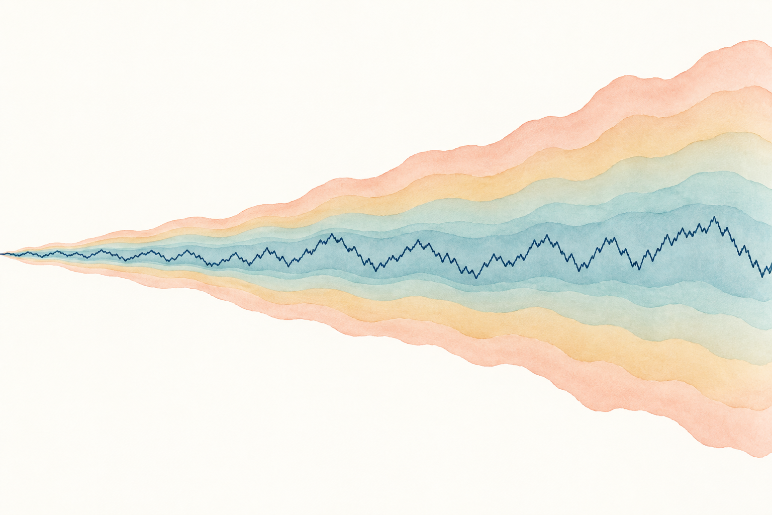
Let \(P_t\) be an observed price and \(x_t=\ln(P_t)\) its log price. A one-period log return is \(r_t=x_t-x_{t-1}\). A \(q\)-period log return adds \(q\) adjacent one-period returns. If those increments are uncorrelated and have stable variance, the variance of the sum grows in proportion to \(q\).

The population variance ratio is

\[ \operatorname{VR}(q)=\frac{\operatorname{Var}(r_t+r_{t-1}+\cdots+r_{t-q+1})}{q\operatorname{Var}(r_t)}. \]

Under that variance-scaling condition, \(\operatorname{VR}(q)=1\). The Lo–MacKinlay procedure turns this relationship into a sample statistic and a test of the random-walk restriction. “One” is the benchmark implied by uncorrelated increments, not a claim that prices are smooth or predictable. Their original application rejected the random-walk specification in historical U.S. equity data, while explicitly cautioning that rejection alone did not establish a mean-reverting price model.

For stationary one-period returns with autocorrelation \(\rho_j\) at lag \(j\), the same population ratio can be written as

\[ \operatorname{VR}(q)=1+2\sum_{j=1}^{q-1}\left(1-\frac{j}{q}\right)\rho_j. \]

Each autocorrelation receives a weight that declines with its lag. The ratio therefore summarizes a weighted set of serial correlations through horizon \(q-1\); it does not equal the autocorrelation at one particular lag.

For \(q=4\), suppose a hypothetical return process has \(\rho_1=0.10\), \(\rho_2=0.04\), and \(\rho_3=0\). Then

\[ \operatorname{VR}(4)=1+2\left(\frac{3}{4}\times0.10+\frac{2}{4}\times0.04\right)=1.17. \]

The value above one reflects positive weighted dependence over those horizons. If the first two autocorrelations were \(-0.10\) and \(-0.04\), with the third still zero, the ratio would be \(0.83\). These are hypothetical population calculations. An observed sample estimate can differ because of sampling variation, changing volatility, and the estimator's finite-sample corrections.

Different autocorrelation patterns can produce the same ratio at one horizon. Positive and negative contributions can offset, so a ratio of exactly one does not require every included autocorrelation to equal zero. Looking at several prespecified horizons can reveal a different pattern, although it also calls for joint inference when the results are tested together.

The test is usually applied to equal-interval log prices or their first differences. If observations are daily closes, \(q=5\) concerns a five-session return, not a calendar week with a different number of trading sessions. Missing sessions, overnight gaps, and irregular timestamps change what “one period” means. State the market calendar and whether prices include distributions or other corporate actions.

Using simple returns instead of log returns is a modeling choice, not a harmless relabeling over every horizon. Log returns add exactly across time; simple returns compound. For small moves they may be numerically close, but the chosen definition should match the question and remain consistent in the example, estimation, and backtest. Never apply the formula to a price level as if it were a return series.

Most implementations form overlapping \(q\)-period returns so that each available observation contributes to the estimate. This increases the number of aggregated observations, but adjacent windows share many one-period returns and are not independent. The test's standard error accounts for this construction under its maintained assumptions; treating the overlapping returns as independent would understate uncertainty.

Suppose a hypothetical asset has a one-session return variance of \(0.0001\), equivalent to a one-session standard deviation of 1%. With uncorrelated increments, a four-session return has variance \(4\times0.0001=0.0004\), so its standard deviation is 2% and the ratio is \(0.0004/(4\times0.0001)=1\).

Now suppose the estimated four-session variance is \(0.000468\), while the one-session estimate remains \(0.0001\). The sample ratio is \(0.000468/(4\times0.0001)=1.17\). That arithmetic describes how dispersion compares across the selected horizons. It does not mean the expected return is 17% larger, that tomorrow's return is 17% more likely to be positive, or that a four-session position has an expected 17% payoff.

To make an inferential claim, compare the estimated ratio with its test distribution and uncertainty estimate. A ratio near 1 can occur even when other aspects of the price process violate a full random-walk model. A ratio away from 1 can also be statistically indistinguishable from 1 in a noisy or short sample. Keep the estimate, test statistic, p-value, and economic interpretation separate.

The classic homoskedastic Lo–MacKinlay statistic studentizes \(\widehat{\operatorname{VR}}(q)-1\) using an asymptotic variance derived under constant-variance increments. If returns have changing conditional volatility, using that standard error can misstate the test size. Lo and MacKinlay also develop a heteroskedasticity-consistent variance estimate for the variance-ratio statistic.

“Heteroskedasticity-consistent” has a specific scope: it adjusts inference for a broader pattern of changing return variance under the test's assumptions. It does not repair a wrong price series, dependence at every possible horizon, structural breaks, stale quotes, or an inadequately short sample. Some software labels the two choices with symbols such as \(Z\) and \(Z^*\); check its documentation to learn which null and standard-error formula it implements.

The 1989 finite-sample study found that performance depends on the null and alternative being considered, and reported better reliability under its heteroskedastic random-walk null than some competing tests in the simulations it examined. That is not a universal guarantee for every sample or implementation. In a small sample, a bootstrap or another finite-sample procedure may be useful, but its resampling design also needs to preserve the dependence and volatility features relevant to the question.

A single-\(q\) test asks whether the variance-scaling restriction holds at one selected horizon. If \(q\) was chosen after inspecting many horizons, the reported p-value does not account for that search. Trying \(q=2,4,8,16\) and highlighting only the most significant result increases the chance of a false positive.

A joint variance-ratio procedure tests a prespecified set of horizons together and adjusts the decision for multiple comparisons. Chow and Denning developed one such multiple test because treating many individual ratios as separate unadjusted decisions can greatly inflate the overall Type I error rate. The joint result is about the tested family of horizons; it does not explain which lag, mechanism, or market participant produced the departure.

Choose horizons for a reason tied to the sampling frequency and research question. A one-day, one-week, and one-month comparison can each be useful, but each has a distinct information set and overlapping-return structure. Report the full tested set, not only the most favorable horizon, and distinguish an exploratory scan from a confirmatory test.

An estimate above one is consistent with positive weighted serial dependence over the selected lags. An estimate below one is consistent with negative weighted dependence over those lags. Neither sign uniquely identifies momentum, mean reversion, delayed price adjustment, inventory effects, bid–ask bounce, nonsynchronous trading, or a volatility process.

In particular, \(\operatorname{VR}(q)<1\) does not prove that the price level is stationary. A series can have a ratio below one at a particular horizon and still contain a stochastic trend. Conversely, rejecting a random-walk restriction does not by itself prove a stationary mean-reverting alternative; Lo and MacKinlay explicitly found that their rejection in the studied equity data did not support that conclusion.

The inference also depends on whether the tested object is a return, log price, excess return, or another transformed series. A result for daily close-to-close returns says nothing automatic about intraday quotes or a different asset universe. State the object and interpretation narrowly.

Bid–ask bounce can create short-horizon negative dependence in transaction-price returns even when a slower economic value process does not reverse. Illiquid securities may update asynchronously, and closing prices can capture different information windows across venues. Those features can affect the shortest horizons most strongly. Check quote quality, trading activity, timestamp alignment, and sensitivity to a slower sampling interval before calling the pattern a market anomaly.

Volatility clustering matters to standard errors even when return signs or levels have no stable directional pattern. A structural change in the mean, volatility, trading hours, or market composition can make one full-sample ratio blend distinct regimes. Inspect subperiod stability without selecting only the window that supports the preferred interpretation.

Searching assets, frequencies, horizons, filters, and sample endpoints creates another problem: selection on noise. A statistically unusual variance ratio found after a broad search is not an untouched hypothesis test. Predeclare a primary horizon or use a suitable joint or resampling method, then validate a discovered pattern in later chronological data.

A variance-ratio test summarizes return variability across horizons. It does not specify direction, entry, exit, stop, position size, holding time, or whether a signal is available before execution. Even a stable dependence pattern may be too small to overcome fees, spread, market impact, funding, borrow, and turnover.

For a trading study, define the signal and decision time before looking at future returns. Estimate any parameters on a formation window, freeze them, and evaluate on later observations. If the result was discovered after trying many securities or horizons, reserve a genuinely untouched test period or use a method that accounts for the search. Compare after-cost results with a baseline and include realistic fills, not just a theoretical return forecast.

Use the variance ratio as one diagnostic alongside plots, autocorrelation checks, unit-root tests, and stability analysis. A variance-scaling departure can motivate a more specific model, but that model needs its own assumptions and out-of-sample evidence. The test is a compact description of a moment restriction, not proof that an edge exists.

State the price definition, return transformation, observation frequency, sample dates, number of usable observations, and whether returns overlap. Report every horizon \(q\) tested, the sample variance ratio, the standard-error version, test statistic, p-value, significance level, and any joint adjustment for multiple horizons.

Explain how missing observations, corporate actions, market closures, and timestamps were handled. Note whether volatility-robust inference, a bootstrap, subperiods, or alternative sampling intervals changed the result. For a trading application, separate the statistical sample from the evaluation period and disclose costs, execution timing, selection rules, and all assets and horizons tried.

Lo and MacKinlay introduce the variance-ratio specification test and study its finite-sample size and power. Chow and Denning explain why testing multiple variance ratios requires joint size control90051-6). For related concepts, see the guides to stationarity and unit roots, Engle–Granger cointegration, and the Johansen cointegration rank test.