Engle–Granger Cointegration Test: Residuals and Error Correction

Two trending series can look related because both contain a stochastic trend. Cointegration is a narrower claim: if the individual series are integrated of order one, I(1), a particular weighted combination may be stationary, I(0). That combination is the long-run equilibrium error under the chosen model. It fluctuates around a stable distribution instead of wandering without bound.

The Engle–Granger two-step procedure is a single-equation way to investigate that claim. In the first step, estimate a long-run relation in levels. In the second, test whether the estimated residual has a unit root. The test is directional in finite samples because the first-stage equation must choose which variable is on the left. This guide follows the classic two-variable setup; it does not replace a system method when several cointegrating relations are possible.

The usual setup assumes the component variables are I(1): their levels are nonstationary under the selected specification, while their first differences are stationary. Unit-root tests are imperfect, especially in short samples and near a structural break, so treat integration-order checks as evidence rather than a mechanical gate. An I(0) series mixed with an I(1) series does not fit the classical I(1)-cointegration case described here.

Decide whether the long-run equation includes an intercept, a deterministic trend, or neither based on the data-generating question. For example, log asset prices might be modeled with an intercept but no deterministic trend in their spread; an economic aggregate may need a trend. The deterministic terms affect both the equilibrium being estimated and the residual-test distribution. Choosing them after looking for a small p-value makes the reported test harder to interpret.

For two level series \(y_t\) and \(x_t\), a simple first-stage equation is

\[ y_t = a + \beta x_t + u_t. \]

Estimate \(a\) and \(\beta\) by ordinary least squares under the maintained assumptions, then save \(\hat u_t = y_t-\hat a-\hat\beta x_t\). If the series are cointegrated in this specification, this fitted combination should be stationary even though the separate levels are not.

In a finance example, \(y_t\) and \(x_t\) could be log total-return indexes for two assets observed at the same frequency. The coefficient \(\hat\beta\) defines the fitted long-run combination; it is not automatically a dollar-neutral or low-risk portfolio weight. Changing the left-hand variable, sample, dividend treatment, currency, or trend specification can change the estimate and the residual. Keep the economic meaning of the equation explicit.

An augmented Dickey–Fuller-style residual regression can be written as

\[ \Delta\hat u_t = \rho\hat u_{t-1} + \sum_{j=1}^{q}\phi_j\Delta\hat u_{t-j} + e_t. \]

The no-cointegration null corresponds to a unit root in the residual; the cointegration alternative is that the fitted residual is stationary. In the simple notation above, evidence against the null comes from a sufficiently negative residual-test statistic. The lag terms help represent serial dependence in the residual, so the lag order and residual diagnostics matter. This is a separate choice from the first-stage intercept or trend used to select the cointegration critical-value case. Too few augmenting lags can leave serial correlation; report how the lag order was chosen and check plausible alternatives, as discussed by Agiakloglou and Newbold.

The residual is estimated in the first step, which changes the null distribution. Do not compare this statistic with ordinary Dickey–Fuller critical values or a generic ADF p-value. Use critical values or p-values designed for the Engle–Granger residual test and the selected deterministic terms, number of variables, and sample size. Phillips and Ouliaris develop the asymptotic theory for residual-based tests; MacKinnon provides response-surface critical values for common specifications.

The same numeric residual-test statistic can face a different reference cutoff when the first-stage deterministic terms or regressor count changes.

Suppose a researcher studies two monthly log-price indexes over a fixed sample. Both appear I(1) under the stated unit-root specifications. The first-stage regression includes an intercept and produces a fitted residual. A residual-based statistic is then evaluated with the Engle–Granger distribution for that deterministic setup and sample—not with the usual ADF table.

Imagine the matching test reports a p-value below the researcher's predeclared 5% threshold. The researcher rejects the null of no cointegration for this specification and finds evidence that the estimated combination is stationary. That conclusion is conditional on the sample, lag choice, deterministic terms, and integration assumptions. It does not show that every pair of assets is related, that the relationship will persist out of sample, or that the fitted residual offers a profitable entry signal. If the p-value were above 5%, the correct reading would be “the test did not reject no cointegration,” not “the series are proven unrelated.”

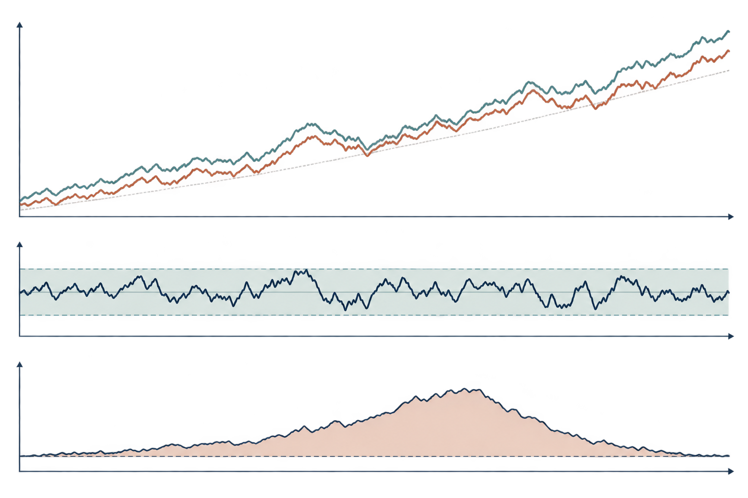
The illustration below is conceptual: common stochastic trends can coexist with a bounded residual, and deviations from a fitted relation can later narrow. It contains no measured series and does not imply that adjustment always occurs at a predictable speed.

If a long-run relation is supported, an error-correction model can combine short-run changes with last period's equilibrium error. With \(\hat u_{t-1}=y_{t-1}-\hat a-\hat\beta x_{t-1}\), one example is

\[ \Delta y_t = c + \lambda\hat u_{t-1} + \sum_{i=1}^{r}\phi_i\Delta y_{t-i} + \sum_{j=0}^{s}\theta_j\Delta x_{t-j} + \epsilon_t. \]

Here \(\lambda\) is the adjustment coefficient for \(y_t\) in this parameterization. If \(y\) is above its fitted relation and \(\lambda<0\), the error-correction term contributes a negative change in \(y\), all else equal. This sign reading uses the definition \(\hat u=y-\hat a-\hat\beta x\); reversing the residual convention reverses the coefficient sign. The short-run coefficients describe additional conditional responses. Another variable may also adjust; cointegration alone does not say which market or economic variable bears the adjustment.

Do not translate \(\lambda\) mechanically into “the spread closes by this percentage each month” unless the model actually has that simple dynamic form. Lagged changes, multiple adjusting variables, nonlinear responses, and breaks affect the path. A stable long-run relation is not a structural causal mechanism, and the adjustment coefficient is conditional on the specified model and information set.

An Engle–Granger single-equation setup can test one proposed long-run combination, including a dependent variable and multiple regressors. With two I(1) variables, the maximum cointegration rank is one; with a larger system, there may be several cointegrating vectors. A single residual test does not determine the full system rank; a Johansen procedure is designed for that rank question under its own VAR and deterministic-term assumptions.

The first-stage normalization also matters in finite samples. Regressing \(y\) on \(x\) is not generally numerically identical to regressing \(x\) on \(y\), even though a long-run relation is conceptually about a combination. Choose the normalization for a clear economic reason and report it. If conclusions change when the equation is reversed, describe that sensitivity rather than selecting the favorable result.

The test can have low power in a small sample, and lag selection, deterministic terms, outliers, and structural breaks can affect its result. A break in the long-run relation can make a previously stationary combination look unstable over the full sample. A single rejection is evidence under a maintained specification, not proof that the relation is permanent.

For a trading application, the fitted residual may be called a spread, but that label does not specify an executable portfolio. A spread built from log prices differs from a dollar-valued position; a price-only series differs from a total-return series. The regression coefficient may drift, and estimated stationarity does not set an entry threshold, holding period, stop, or position size.

Estimate the long-run relation using only data available at each decision date. If you estimate the hedge coefficient using the entire backtest and then trade earlier dates, future observations have leaked into the signal. Use chronological formation and evaluation windows, account for dividends, splits, borrow availability, financing, bid–ask spread, market impact, and rebalancing, and define what happens when diagnostics indicate a break. Search across many pairs and windows also creates selection bias that the cointegration test does not correct.

The practical question is not merely whether one residual test rejects. Ask whether the proposed economic link has a reason to persist, whether it survives a transparent stability check, and whether an implementable rule remains viable after uncertainty and costs. Cointegration can inform a model; it cannot guarantee convergence, hedge effectiveness, or returns.

State the variables, transformations, frequency, sample dates, integration evidence, and first-stage normalization. List the intercept or trend terms, residual-test type, lag-selection rule, test statistic, and the source of the cointegration-specific critical values or p-values. Report sensitivity to a defensible alternative lag or sample window, and note any break analysis.

If you estimate an error-correction model, define the lagged disequilibrium term and sign convention, report which variables are allowed to adjust, and separate short-run coefficients from the long-run relation. For a trading study, disclose chronological splits, pair-selection rules, costs, financing, borrow assumptions, and failure handling. These details distinguish a reproducible test from a chart that only appears to show convergence.

Engle and Granger's original representation, estimation, and testing paper develops the connection between cointegration and error correction. Phillips and Ouliaris derive the asymptotic theory for residual-based cointegration tests. MacKinnon's critical-value study explains response-surface values that depend on sample size and test specification. Agiakloglou and Newbold examine lag structure in the augmented Dickey–Fuller test90022-Q). For a system with multiple possible relations, see Johansen's analysis of cointegration vectors90041-3). Related guides explain cointegration versus correlation in pairs trading, unit roots and mean reversion, and local projections for impulse responses.