The CUSUM Test for Regression Stability and Structural Change

A regression can look reasonable over a full sample even when its relationship changed partway through. Positive prediction errors in one period and negative errors later may cancel in an ordinary full-sample summary. The regression CUSUM test preserves their order: it accumulates recursive prediction errors and checks whether the running path moves too far from the path expected under coefficient stability.

Brown, Durbin, and Evans developed a set of regression stability tools using recursive residuals, including CUSUM and CUSUM of squares. The tests address whether the regression relationship is compatible with constancy over the sample under the model's assumptions. They do not explain why a change occurred, and they are different from industrial process-control CUSUM rules that accumulate deviations from a separately chosen target mean.

This guide focuses on the Brown–Durbin–Evans regression CUSUM. Software may use “CUSUM” for more than one statistic, so a report should name the residual sequence, scaling, boundaries, and reference distribution rather than relying on the label alone.

Write the regression as \(y_t=x_t'\beta+u_t\), where \(x_t\) includes the intercept when the model has one and \(k\) is the number of coefficients. Start with enough observations to estimate the model with full column rank. For each later observation, fit the regression using data only through \(t-1\), then predict \(y_t\).

If \(X_{t-1}\) contains the regressors through the previous observation, the recursive residual is

\[ w_t=\frac{y_t-x_t'\hat\beta_{t-1}}{\sqrt{1+x_t'(X_{t-1}'X_{t-1})^{-1}x_t}},\qquad t=k+1,\ldots,T. \]

The numerator is a one-step prediction error. The denominator adjusts for the leverage-dependent uncertainty of predicting at \(x_t\); it is not an estimate of the market's volatility by itself. Under the classical stable linear model with suitable fixed regressors and independent, equal-variance errors, the recursive residuals have zero mean, are uncorrelated, and share the error variance. Those properties justify accumulating them. They are not guaranteed just because the equation was estimated by least squares.

The initial observations establish the coefficients; they are not a sequence of out-of-sample residuals from this recursion. If the initial design matrix is nearly singular, later predictions can also be unstable. State the initial sample, included regressors, and any transformations because each changes the residual path and the question being tested.

Let \(\hat\sigma\) be the scale estimate used by the selected implementation. The cumulative path through observation \(r\) can be written as

\[ C_r=\frac{1}{\hat\sigma}\sum_{t=k+1}^{r}w_t. \]

Under the stability null, positive and negative innovations should balance over time apart from sampling variation. The plotted path is compared with critical boundaries derived for the test's null distribution. If it crosses a boundary, the test rejects parameter constancy at the chosen level under its assumptions. The exact scaling and boundary construction vary by implementation; a hand-drawn fixed band is not a substitute for the matching critical values.

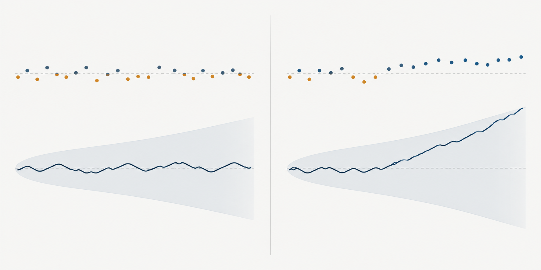
The direction of the path helps explain the pattern. A sustained run of positive recursive errors pushes the sum upward because the observed outcome repeatedly exceeds its prior fitted value. A sustained run of negative errors pushes it downward. Alternating errors can leave the path near its earlier level even when individual residuals are not small. CUSUM therefore uses both the magnitude and the order of prediction errors.

Consider two hypothetical sequences of scale-adjusted recursive residuals. Six values of \(+0.4\) produce a cumulative increase of \(2.4\). The sequence \(+0.4,-0.4,+0.4,-0.4,+0.4,-0.4\) ends at zero. Both contain residuals of the same absolute size, but only the first has persistent direction. These sums illustrate the mechanism; they are not critical values, a p-value, or evidence about a real asset.

The CUSUM of squares uses the squared recursive residuals rather than their signs. A simple cumulative-share form is

\[ Q_r=\frac{\sum_{t=k+1}^{r}w_t^2}{\sum_{t=k+1}^{T}w_t^2}. \]

With a stable equal-variance error process, the cumulative share should grow broadly in proportion to the number of observations. A burst of large squared residuals can make the path steepen; a quiet period can make it flatten. Brown, Durbin, and Evans discuss this alongside the signed CUSUM, while later work studies CUSUM-of-squares tests based on ordinary least-squares residuals.

Do not interpret the squared-residual path as a pure test for volatility or as a clean alternative for coefficient change. Large observations, a variance shift, a misspecified conditional mean, and changing regression coefficients can all affect it. Conversely, the signed CUSUM can be poorly calibrated when variance changes even if positive and negative errors still balance. An ARCH-LM test asks a more specific question about predictability in squared residuals; it still does not diagnose every possible volatility pattern.

The fixed-date Chow test compares regression coefficients on the two sides of a date specified in advance. Regression CUSUM instead examines a recursive path over the ordered sample and does not require one externally specified break date. Its boundary crossing does not give a precise date at which one abrupt change began. A gradual drift, several changes, an outlier sequence, or a variance-model failure may create different path patterns.

When the change date is unknown and the goal is a formal one-break test, Andrews develops supremum Wald, likelihood-ratio, and Lagrange-multiplier procedures with nonstandard critical values. They search over candidate dates while accounting for that search. Their test statistic and critical values are not interchangeable with the Brown–Durbin–Evans CUSUM bands. Tests for multiple breaks require additional procedures and assumptions. See the Chow test guide for the specified-date comparison and Andrews's unknown-change-point paper for the broader search problem.

This distinction matters when an analyst runs many diagnostics. Repeatedly trying CUSUM, CUSUM of squares, candidate dates, regressors, and sample windows creates a selection problem. A nominal level for one prespecified test does not describe the chance of at least one false alarm across all those looks. Record which path or statistic was selected before examining results, or use an inference procedure that accounts for the search.

A retrospective test evaluates a fixed historical sample. A monitoring rule repeatedly evaluates newly arriving data after a baseline period. Applying the same one-shot boundary at every new observation does not automatically preserve its nominal false-alarm rate; the sequence of repeated decisions has a different probability structure.

Chu, Stinchcombe, and White develop fluctuation and CUSUM procedures for real-time monitoring after a historical sample is used to estimate the stable relationship. Their monitoring boundaries address repeated looks under the paper's asymptotic conditions. The baseline must itself be suitable, and the monitoring design must specify what happens after an alert, how parameters are updated, and how long monitoring continues. A historical regression CUSUM chart should not be relabeled as an online procedure without those choices.

For a trading system, an alert means that the model's relationship may no longer match incoming data well enough for the stability assumption to be comfortable. It can trigger investigation or a prespecified risk review. It does not specify which coefficient changed, whether a trade should be placed, or whether reducing exposure will improve returns. If repeated monitoring is used, evaluate detection delay and false-alert costs alongside the statistical threshold.

The classic recursive-residual derivation assumes a correctly specified linear relationship and an error process with stable variance and no serial correlation. Financial time series can violate these conditions through volatility clustering, heavy tails, stale or asynchronous prices, overlapping return horizons, and market-structure changes. A run of residuals can reflect a genuine coefficient shift, omitted dynamics, bad timestamps, or a volatility episode that changes the reference distribution.

Changing the covariance estimator after fitting ordinary least squares does not automatically produce valid CUSUM boundaries. Heteroskedasticity- or dependence-robust inference requires a statistic and reference distribution designed for those conditions. The regression CUSUM plot is a stability diagnostic; it is not a substitute for checking residual dependence, testing conditional heteroskedasticity, or validating the specification. Continue with the ARCH-LM test guide and the robust standard errors guide when those questions are relevant.

Choose the sampling interval and market calendar before constructing residuals. A close-to-close return spanning a long holiday is not the same interval as an ordinary session return. Corporate actions, contract rolls, currency conversion, and missing observations can also create prediction errors that resemble instability. Do not fill gaps or align assets mechanically without explaining what the model's observation at time \(t\) represents.

Name the outcome, regressors, intercept, transformations, sample dates, frequency, initial estimation period, and number of recursive residuals. State whether residuals were scaled by a recursive prediction variance and how \(\hat\sigma\) was estimated. Identify the CUSUM or CUSUM-of-squares version, the reference distribution, critical level, boundary rule, and any software defaults that affect them.

Show the path or statistic alongside the fitted coefficients and residual diagnostics. A boundary crossing is evidence against constancy under the tested model, not an estimate of the economic cause or a causal effect of a named event. If the purpose is forecasting or trading, use chronological holdouts, disclose when each alert would have been available, and account for spread, market impact, fees, borrow, financing, and turnover. Compare the response with a fixed-model benchmark. A stability warning can motivate a model review; it does not demonstrate that an adaptive rule has an edge.

Brown, Durbin, and Evans introduce the recursive-residual CUSUM and CUSUM-of-squares stability procedures in their 1975 paper. McCabe and Harrison study a CUSUM-of-squares test using ordinary least-squares residuals. For unknown change points, see Andrews (1993); for sequential monitoring, see Chu, Stinchcombe, and White (1996). Related guides cover OLS regression, the Chow test, and volatility clustering.