The Chow Test for Structural Breaks in Regression

A regression fitted over a long sample can hide a change in the relationship between an outcome and its predictors. For example, a portfolio’s estimated exposure to a broad market return may differ before and after a market-structure change. The Chow test turns that question into a joint hypothesis about regression coefficients on the two sides of a specified date.

Suppose the model has k coefficients, including its intercept. The null is that the pre-break coefficient vector and post-break coefficient vector are equal. The alternative is that at least one tested coefficient differs. The original 1960 paper by Gregory Chow frames this as testing equality between coefficient sets from two linear regressions; see Chow’s paper.

“Structural break” is shorthand for a change in the conditional relationship represented by the chosen model. The test does not show that every part of the data-generating process changed, and it does not identify a cause. A rejection is evidence against the tested stability restriction for the selected sample, model, and date. A non-rejection is not proof that the relationship is permanently stable.

Let y be the outcome and x contain an intercept and the included explanatory variables. A pooled regression imposes one coefficient vector across the whole sample. To allow a post-date change, define D as zero before the break and one after it, then interact D with each regressor: y = x′β + D·x′δ + u. The pre-break vector is β; the post-break vector is β + δ.

The full stability null is H₀: δ = 0, a joint restriction covering the intercept and all slopes in the specified model. For a regression with an intercept and two predictors, k = 3. If the question concerns only a market beta, test only the interaction attached to that market-return predictor; do not silently turn that narrower question into a test of every coefficient.

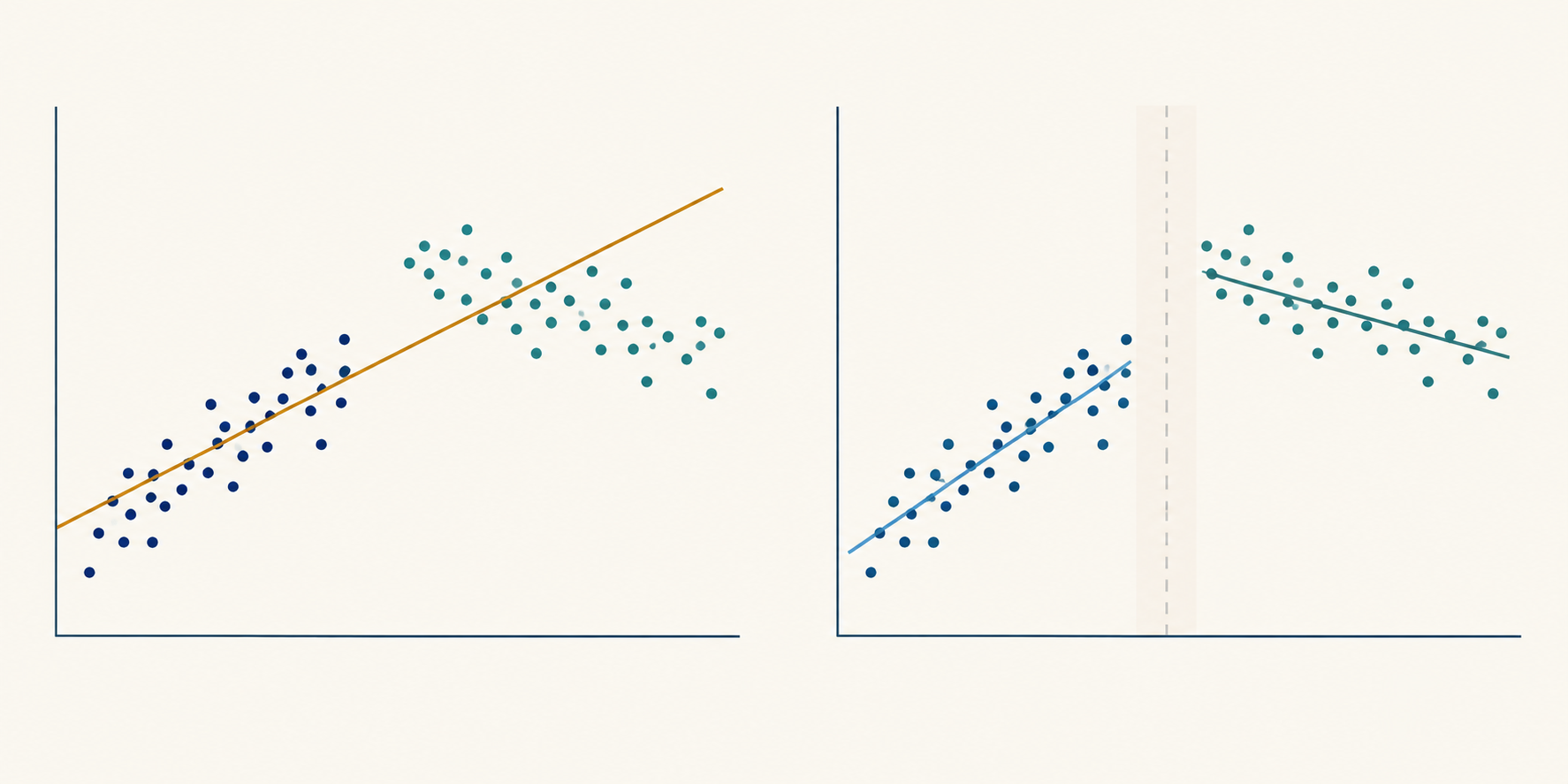
This interaction form explains what the split-regression calculation tests. The pooled regression is the restricted model, with pre- and post-break coefficients forced to match. The two separate regressions are the unrestricted model, with their coefficient vectors estimated independently. The two approaches test the same full-equality null when they use the same observations, regressors, and restrictions.

<!-- Illustration placeholder: A text-free conceptual scene showing one cloud of observations split by a clear vertical time boundary, with one shared fitted relationship above and two different fitted relationships below. No words, labels, numeric values, axes text, logos, or interface elements. -->

The classical Chow setup treats the break date as supplied. A date can be motivated by an external rule change, a known contract redesign, a data-definition change, or another event whose timing was determined independently of the outcome. The study still needs to state how observations on the date itself are assigned and whether returns, releases, and exchange sessions are aligned consistently.

A fixed-date Chow test represents one abrupt change. An announced rule may be anticipated before its formal start, a rollout may be phased in, or trading conditions may change more than once. Distinguish the announcement, effective, and actual implementation dates according to the mechanism that could alter the measured relationship. If a gradual response is part of the prespecified question, a ramp or distributed interaction may fit better than a single step indicator. Choosing that shape after comparing which one produces the smallest p-value introduces another search.

If a researcher tries many dates and reports the one with the largest F statistic, the reported statistic is selected from a search. Its ordinary single-date F reference distribution no longer accounts for that selection. Repeating the test across many assets, outcomes, sample windows, or predictor sets creates the same problem: the most striking result can partly reflect the search rather than instability.

When the change point is unknown, use a procedure designed for that question. Andrews’s work on parameter instability with an unknown change point shows why the resulting test has a nonstandard null distribution; its critical values are not simply the usual fixed-date Chow F cutoff. For multiple unknown changes, Bai and Perron develop procedures for testing and estimating multiple break dates. These methods have their own assumptions and trimming choices, so they are not automatic fixes for every time series. See Andrews (1993) and Bai and Perron (1998).

Fit one pooled regression and record its residual sum of squares, SSRₚ. Then fit a regression on each side of the specified date and record SSR₁ and SSR₂. When the full coefficient vector is allowed to differ, the classical statistic is F = [(SSRₚ − SSR₁ − SSR₂) / k] ÷ [(SSR₁ + SSR₂) / (n₁ + n₂ − 2k)]. Here, n₁ and n₂ are the observations in each group, and k is the number of coefficients estimated in each group, including the intercept.

The numerator measures the pooled model’s extra squared error after imposing k equality restrictions, divided by the number of restrictions. The denominator estimates the common residual variance using the split model’s residual degrees of freedom. The reference distribution is F with k numerator degrees of freedom and n₁ + n₂ − 2k denominator degrees of freedom. The split regressions must have enough independent information to estimate their k coefficients; rank deficiency makes the comparison unusable.

This formula is for testing all k coefficients at once under the classical linear-model conditions, including independent, normally distributed errors with the same variance in both groups. If only q restrictions are tested, use a valid restricted-versus-unrestricted joint F test with q numerator degrees of freedom; do not substitute q into the full split-SSR formula while leaving its models unchanged. In a design matrix with interactions, a joint Wald test is the corresponding general way to state the restrictions.

Imagine a researcher asks whether a portfolio’s weekly return relationship to a market factor and a second risk factor changed after a date chosen in advance because of a hypothetical exchange rule change. The fitted model has an intercept and two factor slopes, so k = 3. Suppose there are n₁ = 80 pre-date observations and n₂ = 100 post-date observations. All figures in this example are invented and are not market estimates.

Assume the pooled regression has SSRₚ = 360 basis-points-squared, while the two split regressions have SSR₁ = 130 and SSR₂ = 150. The pooled restriction increases SSR by 360 − 130 − 150 = 80. The numerator is 80 / 3 = 26.67. The split-model residual degrees of freedom are 80 + 100 − 2 × 3 = 174, so the denominator is 280 / 174 ≈ 1.609. The resulting statistic is F(3, 174) ≈ 16.57, with a conventional upper-tail p-value of about 1.6 × 10⁻⁹ under the stated classical assumptions. The 5% critical value is about 2.66, so this hypothetical calculation rejects full coefficient stability.

That conclusion is deliberately narrow: at least one coefficient in this model differs across the two samples, assuming the model and error conditions are suitable. The statistic does not say whether the market beta rose or fell; that requires inspecting the estimates and their uncertainty. It does not show the rule change caused the difference, and it says nothing by itself about post-break expected returns, implementable forecasts, or net strategy performance.

An intercept shift can mean the conditional average of y moved after controlling for the included predictors. A slope shift can mean the outcome’s estimated response to a predictor changed. The full Chow test combines these possibilities. A rejection tells the reader that the equality of the tested coefficient vector is not supported; it does not identify the coefficient responsible unless the estimates and additional, properly specified restrictions are examined.

Testing each coefficient separately is not a substitute for the joint test. Several modest shifts can be jointly inconsistent with equality even if no single coefficient test is decisive. Conversely, a significant individual coefficient after looking at many possible terms may be a multiple-testing result. State the joint hypothesis first, then report coefficient estimates, confidence intervals, and economically meaningful contrasts for the parameters that answer the research question.

A Chow test also differs from interrupted-time-series analysis. The latter models a pre-intervention trajectory and estimates a level and/or trend change relative to that path. Chow’s test asks whether specified regression coefficients match across groups; by itself it does not build an intervention counterfactual. A break near an event date may still reflect another simultaneous shock, a change in sample composition, or a revised measurement process. The existing interrupted-time-series guide covers intervention paths; a coefficient difference alone is not causal identification.

For a research-design treatment of interrupted time series, see Bernal, Cummins, and Gasparrini’s review.

The simple Chow F reference can be misleading when errors are serially correlated, heteroskedastic, or otherwise inconsistent with its common-variance model. Financial returns often have changing conditional variance; neighboring observations may share information or shocks, and observations around a market closure can have a different interpretation from ordinary adjacent sessions. A visually plausible break does not make the conventional error assumptions true.

Separate a change in the conditional mean relationship from a change in residual variance. If the slopes are stable but the error variance differs across regimes, the common-variance assumption fails; the classical split-SSR statistic can then look like evidence about coefficient stability for the wrong reason. Conversely, a robust covariance estimator changes the uncertainty calculation but is not itself a test that the coefficients are stable. Inspect both the interaction restrictions and residual scale rather than treating those as one diagnostic question.

One option is to express the break with interactions in a pooled regression and test the chosen coefficient restrictions using a covariance estimator appropriate for the data. White’s heteroskedasticity-consistent covariance estimator addresses a different error variance pattern than the classical formula; Newey and West’s HAC estimator allows heteroskedasticity and autocorrelation under its conditions. These do not preserve the exact classical finite-sample F distribution. The robust Wald statistic usually relies on an asymptotic approximation, and lag or bandwidth choices still need justification. See White’s covariance paper and Newey–West.

A robust covariance estimator does not repair omitted predictors, a poorly chosen functional form, endogenous regressors, a break date selected from the same outcome series, or too few observations in either regime. Check residual dependence, variance changes, influential observations, and stability to defensible windows. If the dependent variable or regressors are nonstationary, establish what the regression represents before treating a significant break statistic as meaningful evidence about a stable relationship.

A reproducible report identifies the outcome, predictors, transformations, sample frequency, observation counts on each side, exact break-date rule, and all coefficient restrictions. For the classical calculation, include the pooled and separate SSR values, k, degrees of freedom, F statistic, p-value, and error assumptions. For a robust interaction test, name the covariance estimator, its tuning choices, and whether inference uses a finite-sample or asymptotic reference distribution.

Show the pre- and post-break coefficient estimates with uncertainty, not only the rejection label. Explain whether the estimated difference is economically material, whether it survives sensible alternative windows and predictor definitions, and whether the date was prespecified or searched. A break in coefficients can motivate model review, re-estimation, or a monitoring rule, but it does not itself prove that a trading strategy should be changed or that a new strategy will work.

For a forecasting or trading application, test the response using information available at each historical decision time. Compare forecasts or portfolio outcomes out of sample with a clear benchmark and include turnover, spreads, fees, funding where relevant, and capacity constraints. A statistically significant in-sample break is a diagnostic about model stability, not evidence of future alpha. For background on regression interpretation, continue with the OLS guide; for inference with dependent errors, see the robust-standard-errors guide.