Pre-Averaging Realized Volatility: Microstructure Noise का Estimator

अगर observed price बिल्कुल efficient price होता, तो intraday returns के squares जोड़ना session की variation estimate करने का स्वाभाविक तरीका होता। लेकिन transaction prices और quotes में bid–ask bounce, tick-size rounding, latency, discrete price levels या recording conventions का असर हो सकता है। Sampling interval बहुत छोटा होने पर हर squared return का बड़ा हिस्सा इन प्रभावों से आ सकता है। अधिक observations जोड़ने से केवल latent price की नई movement सामने आए, यह जरूरी नहीं; noise contribution भी बढ़ सकता है।

Pre-averaging इस समस्या के लिए return square करने से पहले उन्हें छोटी local window में जोड़ता है। Smooth weight function शून्य से शुरू होता है, पास के returns को weight देता है और window के अंत में फिर शून्य हो जाता है। Weighted sum local filter की तरह काम करता है: तेज़ी से बदलने वाली independent observation errors कुछ हद तक cancel हो सकती हैं, जबकि efficient price की व्यापक movement बच सकती है। Overlapping windows पूरे interval में सूचना का उपयोग करती हैं।

सिर्फ smoothing से estimator unbiased नहीं हो जाता। Filtered returns के squares में noise variation बचती है, इसलिए correction term चाहिए। Jacod, Li, Mykland, Podolskij और Vetter ने स्पष्ट assumptions के तहत integrated volatility estimate करने के लिए pre-averaging method निकाली और दिखाया कि उपयुक्त रूप \(n^{-1/4}\) convergence rate पा सकते हैं। उनका मूल शोधपत्र method का आधार है; यह guide इसकी mechanics, choices और limits समझाता है।

Observation time \(t_i\) पर latent efficient log price को \(X_{t_i}\) और recorded log price को \(Y_{t_i}\) लिखें:

\[ Y_{t_i}=X_{t_i}+\epsilon_{t_i}, \]

जहाँ \(\epsilon_{t_i}\) observation noise है। एक सामान्य baseline model में \(X_t\), local variance rate \(\sigma_t^2\) वाला continuous semimartingale है। निश्चित interval \([0,T]\) के लिए target integrated variance है:

\[ IV_T=\int_0^T \sigma_t^2\,dt. \]

Observed return को \(\Delta_iY=\Delta_iX+\epsilon_{t_i}-\epsilon_{t_{i-1}}\) लिखा जा सकता है। Price errors observations के बीच independent हों तब भी पास-पास के दो returns एक endpoint error को विपरीत signs के साथ share करते हैं। इससे returns में serial dependence आती है और सभी observations वाला realized variance noisy differences की संख्या के प्रति sensitive होता है।

सरल theoretical explanation में अक्सर zero-mean noise माना जाता है, जो समय के साथ और efficient-price process से independent हो तथा उसके moments finite हों। Correction का स्रोत समझने में यह उपयोगी है, लेकिन trades, quotes या midpoint prices में इसकी गारंटी नहीं। Noise liquidity और दिन के समय के साथ बदल सकता है, efficient price से जुड़ सकता है या serially dependent हो सकता है। Target भी स्पष्ट करें: jumps हों तो quadratic variation में jump squares शामिल होते हैं, जबकि continuous integrated variance में नहीं।

यह एक तय price series और समयावधि का ex post measurement है। यह हर latent price फिर से नहीं बनाता, किसी एक गलत print को चिन्हित नहीं करता और भविष्य की volatility नहीं बताता। Estimates की तुलना से पहले बताएं कि input transaction prices, quote midpoints या कोई दूसरी price construction है।

\(n\) observed returns \(r_i=Y_{t_i}-Y_{t_{i-1}}\) के लिए integer window length \(k_n\) और \([0,1]\) पर weight function \(g\) चुनें। एक सामान्य pre-averaged return है

\[ \bar r_i=\sum_{j=1}^{k_n-1}g\!\left(\frac{j}{k_n}\right)r_{i+j}, \qquad i=0,\ldots,n-k_n+1. \]

आमतौर पर function continuous होता है, दोनों सिरों पर शून्य होता है और asymptotic results के लिए पर्याप्त smooth रहता है। Triangular उदाहरण \(g(u)=\min(u,1-u)\) है। Window के दोनों छोर पर weight शून्य होने से किनारे का return अचानक पूरा weight नहीं पाता। यह स्थानीय weight shape है, forecast या fitted trend नहीं।

हर \(\bar r_i\) आस-पास के returns को square करने से पहले जोड़ता है। Windows overlap करती हैं, इसलिए raw returns independent हों तब भी pre-averaged returns correlated होते हैं। यह dependence estimator के sampling behavior का हिस्सा है; बहुत सी window sums को independent observations नहीं मानना चाहिए। Index range और endpoint convention को weight normalization से मेल खाना चाहिए।

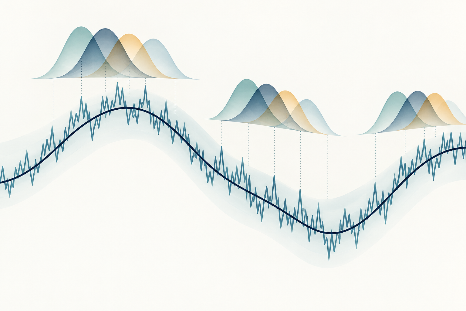
चित्र में smooth latent path, उसके आसपास jagged observed path और tapering weights वाली कई overlapping windows हैं। यह local pooling समझाने के लिए है; price record या empirical filter output नहीं।

<!-- learn:illustration --> <!-- Text-free concept: smooth latent price path के पास jagged observed path और पड़ोसी movements को जोड़ती overlapping tapered local windows। यह अवधारणात्मक है, market data, forecast या trading signal नहीं। -->

Pre-averaging तेज़ observation errors का असर घटाता है, पर filtered returns के squares में noise contribution रहती है। Regular grid के लिए asymptotic normalizers वाला univariate estimator का एक सामान्य रूप है

\[ \widehat{IV}_{PA} =\frac{1}{k_n\psi_2}\sum_{i=0}^{n-k_n+1}\bar r_i^2 -\frac{\psi_1}{2\psi_2 k_n^2}\sum_{i=1}^{n}r_i^2, \]

जहाँ weight constants हैं

\[ \psi_1=\int_0^1 \{g'(u)\}^2\,du, \qquad \psi_2=\int_0^1 g(u)^2\,du. \]

पहला term pre-averaged squared returns के sum को integrated variance के scale पर लाता है। दूसरा, model के तहत, observation noise की leading contribution estimate करके घटाता है। यह noise की हर realization estimate नहीं करता और गलत price field, timestamp error या outlier को ठीक नहीं करता। Finite-sample formula में \(\psi_1,\psi_2\) के discrete versions, endpoint adjustments और return indexing की खास convention हो सकती है। इन बातों को बताएं और लगातार एक ही convention अपनाएँ।

Correction के बाद finite-sample estimate छोटा या negative हो सकता है। इसका अर्थ asset की physical variance negative होना नहीं है; उस sample में चुना गया correction पहले term से बड़ा था। Negative estimate को चुपचाप zero न करें। Raw calculation और अलग truncation rule हो तो दोनों बताएं, क्योंकि truncation estimator बदलता है और आगे की averages या inference पर असर डाल सकता है।

\(k_n\) smoothing की मात्रा नियंत्रित करता है। Window बहुत छोटी हो तो filtered returns में high-frequency noise अधिक बचता है। Window बहुत लंबी हो तो local price movements लंबे समय में average होते हैं और कम windows योगदान देती हैं, जिससे दूसरी तरह की estimation error बढ़ सकती है। Window length और weight function साथ काम करते हैं; weight shape और sampling interval के बिना \(k_n\) का अर्थ नहीं है।

Classical balanced design में, fixed time span के भीतर \(n\) तेजी से sampled observations बढ़ने पर window का order \(\sqrt n\) होता है; इसे अक्सर positive tuning constant \(\theta\) के लिए \(k_n\sim\theta\sqrt n\) लिखा जाता है। Paper की assumptions के तहत estimator \(n^{1/4}\) rate से converge कर सकता है, यानी estimation error \(n^{-1/4}\) के order का होता है। यह noise-free \(n^{1/2}\) rate से धीमा है और लेखकों के baseline noisy setting में optimal है; हर market dataset के लिए guarantee नहीं।

\(\theta\), weight function और data-driven selection method finite-sample bias तथा variance को प्रभावित करते हैं। Automatic choice noise और volatility estimates पर निर्भर हो सकती है, जिनमें स्वयं uncertainty है। उचित window choices में sensitivity दिखाएं, sampling clock और session boundaries बताएं, और पसंदीदा निष्कर्ष के अनुकूल value देखकर window न चुनें।

Basis points में छह hypothetical observed returns मानें:

\[ (r_1,\ldots,r_6)=(1,0,1,0,1,0)\ \mathrm{bp}. \]

Triangular weight \(g(u)=\min(u,1-u)\) और जानबूझकर छोटी window \(k=3\) लें। दो अंदरूनी grid weights \(g(1/3)=g(2/3)=1/3\) हैं। इस छोटी grid पर arithmetic साफ दिखाने के लिए discrete normalizers परिभाषित करें:

\[ \psi_{2,k}=\frac{1}{k}\sum_{j=1}^{k-1}g(j/k)^2=\frac{2}{27}, \qquad \psi_{1,k}=k\sum_{j=1}^{k}\{g(j/k)-g((j-1)/k)\}^2=\frac{2}{3}. \]

ऊपर वाली index convention के अनुसार \(n-k+2=5\) overlapping windows हैं। हर window पड़ोसी \(1\) bp और \(0\) bp return जोड़ती है, इसलिए \(\bar r_i=(1/3)(1+0)=1/3\) bp और

\[ \sum_i\bar r_i^2=5\left(\frac13\right)^2=\frac59\ \mathrm{bp}^2, \qquad \sum_{i=1}^{6}r_i^2=3\ \mathrm{bp}^2. \]

उचित discrete normalization रखने पर

\[ \widehat{IV}_{PA} =\frac{1}{3(2/27)}\left(\frac59\right) -\frac{2/3}{2(2/27)3^2}(3) =2.5-1.5=1\ \mathrm{bp}^2. \]

यह उदाहरण arithmetic और units जाँचने के लिए है; छह returns और इतना छोटा window asymptotic approximation का समर्थन नहीं करते। संख्याएँ गणना स्पष्ट करने के लिए बनाई गई हैं। ये market data, noise-process simulation या latent integrated variance recover होने का प्रमाण नहीं हैं। Standard error या forecast नहीं निकाला गया।

Standard derivation में continuous efficient-price process, additive noise, frequent observations और कुछ regularity conditions माने जाते हैं। Zero-mean independent noise उपयोगी शुरुआत है, लेकिन noise और price के बीच dependence, serially correlated errors, समय के साथ बदलता noise, irregular observation times या endogenous sampling के लिए modified estimator या उसी परिस्थिति की theory चाहिए हो सकती है। Aït-Sahalia, Mykland और Zhang dependent microstructure noise के साथ integrated volatility estimation का अध्ययन करते हैं। उनका शोधपत्र बताता है कि independent-noise formula सार्वभौमिक नहीं है।

Jumps हों तो target पर अलग निर्णय चाहिए। Quadratic variation में jump squares शामिल होते हैं, continuous integrated variance में नहीं। साधारण pre-averaging estimator jumps को अपने-आप अलग नहीं करता। Jump-robust truncation या दूसरी construction की अपनी assumptions और tuning हैं। एक बड़ा bad print कई overlapping windows को भी प्रभावित कर सकता है, इसलिए data validation और outlier handling जरूरी रहती है।

Pre-averaging अकेले multivariate या asynchronous data की सारी समस्याएँ भी नहीं सुलझाता। Christensen, Kinnebrock और Podolskij non-synchronous observations के लिए pre-averaging covariance methods और noise-robust Hayashi–Yoshida extension विकसित करते हैं (अध्ययन). ये constructions sampling design के अतिरिक्त मुद्दे संभालते हैं। हर asset पर univariate formula अलग से लगाने से timestamps अपने-आप synchronize नहीं होते और valid covariance matrix की guarantee नहीं मिलती।

ये estimators high-frequency variation की संबंधित समस्याएँ हल करते हैं, लेकिन सूचना को अलग ढंग से व्यवस्थित करते हैं। Two-scale realized volatility यानी TSRV shifted sparse sampling grids पर realized variance average करता है, फिर leading noise bias correct करने के लिए fine-grid estimate का scaled हिस्सा घटाता है। Pre-averaging इसके बजाय smooth weights से छोटे overlapping return windows filter करता है, filtered returns को square करता है और उससे मेल खाता correction लगाता है। मूल two-scale paper अलग construction बताता है।

Realized kernel squared-return sum से शुरू होकर कई lags पर weighted return autocovariances जोड़ता है। Bandwidth तय करता है कि सबसे दूर का lag कौन सा होगा। Pre-averaging returns को square करने से पहले local returns बदलता है। दोनों में weights और tuning choices हैं, लेकिन उनके formulas, normalization और assumptions परस्पर interchangeable नहीं हैं। Lag-based construction और bandwidth के लिए realized-kernel guide देखें।

Method का नाम नहीं, data और जरूरी target देखकर चुनाव करें। Sampling design, noise model, endpoint handling, jump target और finite-sample behavior की तुलना करें। Asymptotic noise robustness का अर्थ यह नहीं कि illiquid assets, छोटी session, बदलते noise या irregular data feed में वही सबसे अच्छा होगा। TSRV guide उसके scale और correction choices समझाता है।

Result दोहराया जा सके, इसके लिए asset और price field, interval, sampling frequency, timestamp तथा session rules, return units, weight function, window length, normalization, endpoint convention और noise assumptions बताएं। Inference के लिए estimator इस्तेमाल हो तो variance estimator या confidence procedure और उनकी assumptions भी रिपोर्ट करें। उचित window lengths के across sensitivity table से दिख सकता है कि निष्कर्ष किसी एक tuning choice पर निर्भर है या नहीं।

Integrated variance पूरा हो चुका observed interval मापता है। इसका square root उसी interval का volatility scale देता है, forecast नहीं। Annualization के लिए स्पष्ट time convention चाहिए और इससे भी forecast नहीं बनता। भविष्य की अवधि का forecast अलग predictive model और out-of-sample evaluation माँगता है। Basic squared-return benchmark के लिए realized-volatility calculation guide देखें; path variation और continuous integrated-variance target का फर्क quadratic-variation guide समझाती है।

Estimate यह साबित नहीं करता कि price क्यों बदला, profitable strategy नहीं पहचानता और executable risk सही मापने की guarantee नहीं देता। Trading costs, liquidity, jumps, volatility dynamics और estimator uncertainty अलग प्रश्न हैं। Pre-averaging एक statistical measurement tool है; इसकी उपयोगिता इस पर निर्भर करती है कि स्पष्ट assumptions observed data से कितनी मेल खाती हैं।