Time-Series Autocorrelation के लिए Ljung–Box Test

Sample autocorrelation plot कई lags पर dependence दिखा सकता है, लेकिन बहुत सी bars को अलग-अलग पढ़ने से multiple-testing समस्या पैदा होती है। Ljung–Box test पहले \(h\) sample autocorrelations को एक portmanteau statistic में जोड़ता है। इसका null है कि lag 1 से \(h\) तक सभी population autocorrelations शून्य हैं। Alternative है कि कम-से-कम एक correlation शून्य से अलग है।

Box और Pierce ने fitted time-series models के लिए overall lack-of-fit test बनाया। Ljung और Box ने finite samples में approximation बेहतर करने के लिए statistic बदला। “Portmanteau” का अर्थ है कि एक statistic कई lag-specific correlations का सार देता है; इसका अर्थ यह नहीं कि time-series dependence के हर प्रकार की जाँच हो गई।

Return series पर सवाल हो सकता है कि पुराने signed returns linear serial dependence छोड़ते हैं या नहीं। Fitted ARMA model पर आम सवाल है कि बताई गई lag structure इस्तेमाल करने के बाद residual autocorrelation बची या नहीं। ये जुड़े हुए, लेकिन अलग उपयोग हैं; नतीजा समझने से पहले बताएँ कि किस series को जाँचा।

Lag \(k\) पर sample autocorrelation \(\hat\rho_k\), उसकी गणना में प्रयुक्त observations की संख्या \(n\), और test का सबसे बड़ा lag \(h\) मानें। Box–Pierce statistic है:

\[ Q_{BP}=n\sum_{k=1}^{h}\hat\rho_k^2. \]

Ljung–Box adjustment हर lag पर उपलब्ध sample size के अनुसार weight देता है:

\[ Q_{LB}=n(n+2)\sum_{k=1}^{h}\frac{\hat\rho_k^2}{n-k}. \]

Correlations को square करने से positive और negative autocorrelation दोनों statistic बढ़ाते हैं। Adjustment, समान estimated correlation के लिए उन lags को ज्यादा weight देता है जहाँ usable pairs कम हैं। बड़े samples में दोनों statistics अक्सर करीब आ जाते हैं; finite samples में Ljung–Box आम है क्योंकि मूल अध्ययन में इसका small-sample approximation बेहतर था।

White-noise null और test की regularity conditions के तहत \(Q_{LB}\) की तुलना chi-square distribution से की जाती है। कोई dynamic parameter fit न किए गए raw series के लिए reference degrees of freedom आम तौर पर \(h\) हैं। अनुमानित ARMA(\(p,q\)) model residuals के लिए आम adjustment \(h-p-q\) है, बशर्ते यह धनात्मक हो। यह correction residual dynamics fit करने में इस्तेमाल parameters को दर्शाता है; हर regression से हर coefficient घटाने का सार्वभौमिक निर्देश नहीं। Integrated, seasonal, constrained या अन्य विशेष models के लिए अलग conventions हो सकती हैं। Reference degrees of freedom को वास्तविक residual test और software definition से मिलाएँ। उदाहरण के लिए, ARMA(2,2) residuals को केवल \(h=4\) तक जाँचने पर आम adjustment में degrees of freedom शून्य हैं। तब सामान्य chi-square comparison उपलब्ध नहीं है। Zero-degree reference को जबरन लगाने के बजाय पहले से लंबा lag range चुनें या उस model के लिए बने diagnostic का उपयोग करें। Lag horizon चुनने का कारण भी बताएँ।

मान लें fitted model से \(n=250\) residuals बचे और पहले से चुने गए पाँच-lag check में autocorrelations \(0.10, 0.05, -0.08, 0.02, -0.04\) आए। Box–Pierce में पहले उन्हें square करके जोड़ते हैं:

\[ 0.10^2+0.05^2+(-0.08)^2+0.02^2+(-0.04)^2=0.0209. \]

इसलिए \(Q_{BP}=250(0.0209)=5.225\)। Ljung–Box weights लगाने पर

\[ Q_{LB}=250(252)\left(\frac{0.0100}{249}+\frac{0.0025}{248}+\frac{0.0064}{247}+\frac{0.0004}{246}+\frac{0.0016}{245}\right)\approx 5.31. \]

यह गणना अभी p-value नहीं है। यदि ये ARMA(1,1) fit के residuals हैं, तो आम reference \(h-p-q=5-1-1=3\) degrees of freedom इस्तेमाल करता है; raw series अपनी null के तहत पाँच ले सकता है। Degrees of freedom चुनने से upper-tail probability बदलती है। यहाँ सभी संख्याएँ हिसाब समझाने के लिए काल्पनिक हैं, market data या model result नहीं।

छोटा statistic बताता है कि चुने हुए reference distribution में observed squared autocorrelations असामान्य रूप से बड़े नहीं हैं। यह साबित नहीं करता कि correlations ठीक शून्य हैं। बड़ा statistic कहता है कि चुने गए level पर set को null से मेल कराना कठिन है; एक संख्या को diagnosis न मानें, देखें कि कौन-से lags और model features इसके लिए जिम्मेदार हैं।

Lag limit \(h\) test का प्रश्न तय करता है। कुछ छोटे lags जाँचने से धीमी dependence या daily observations में weekly pattern छूट सकता है। बहुत सारे lags जोड़ने से कमजोर, noisy estimates बढ़ सकते हैं, किसी विशिष्ट short-lag pattern के खिलाफ power घट सकती है और परिणाम कुछ long-lag correlations के प्रति संवेदनशील हो सकता है। बड़े \(h\) पर ARMA adjustment के बाद degrees of freedom भी कम बचते हैं।

Sampling frequency, ज्ञात calendar structure, model का उद्देश्य और residuals में अब कौन-सी dependence नहीं रहनी चाहिए—इन आधारों पर lags चुनें। Daily market data में trading-session lag हमेशा calendar-day lag जैसा नहीं होता। Intraday data में time-of-day और overnight effects हो सकते हैं। Seasonal model में seasonal lags या खास diagnostic चाहिए; एक generic cutoff ऐसी structure छिपा सकता है।

यदि कई \(h\), transformations, assets या model orders आजमाकर सिर्फ सबसे छोटा p-value रिपोर्ट किया जाता है, तो दिखाई गई significance search को नज़रअंदाज़ करती है। Diagnostic समझने से पहले lag range और decision rule तय करें, या broader search को inference plan में शामिल करें।

Autocorrelation plot में अक्सर \(\pm1.96/\sqrt{n}\) जैसी approximate single-lag bands होती हैं। Simple white-noise model में वे individual sample correlation को flag कर सकती हैं, लेकिन हर lag के लिए simultaneous 95% band नहीं हैं। कई bars अलग-अलग देखने पर कम-से-कम एक के संयोग से पार होने की संभावना बढ़ती है। Ljung–Box इसके बजाय prespecified set पर एक joint question पूछता है और combined statistic का reference distribution इस्तेमाल करता है।

एक अपेक्षाकृत बड़ा autocorrelation या कई मामूली correlations—दोनों joint statistic बढ़ा सकते हैं। Test के बाद lag-by-lag terms \(n(n+2)\hat\rho_k^2/(n-k)\) और ACF plot देखें। Heuristic band के बाहर एक bar अपने-आप significant portmanteau result नहीं है; हर अलग band के अंदर bars होने से joint statistic के insignificant होने की गारंटी भी नहीं मिलती।


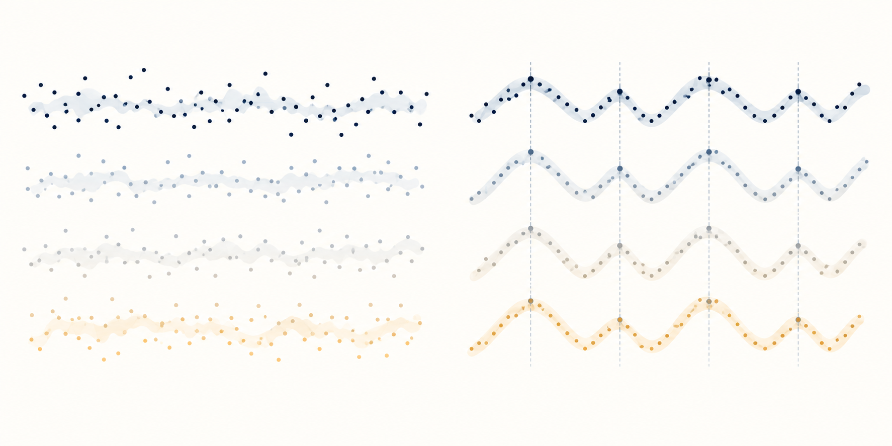
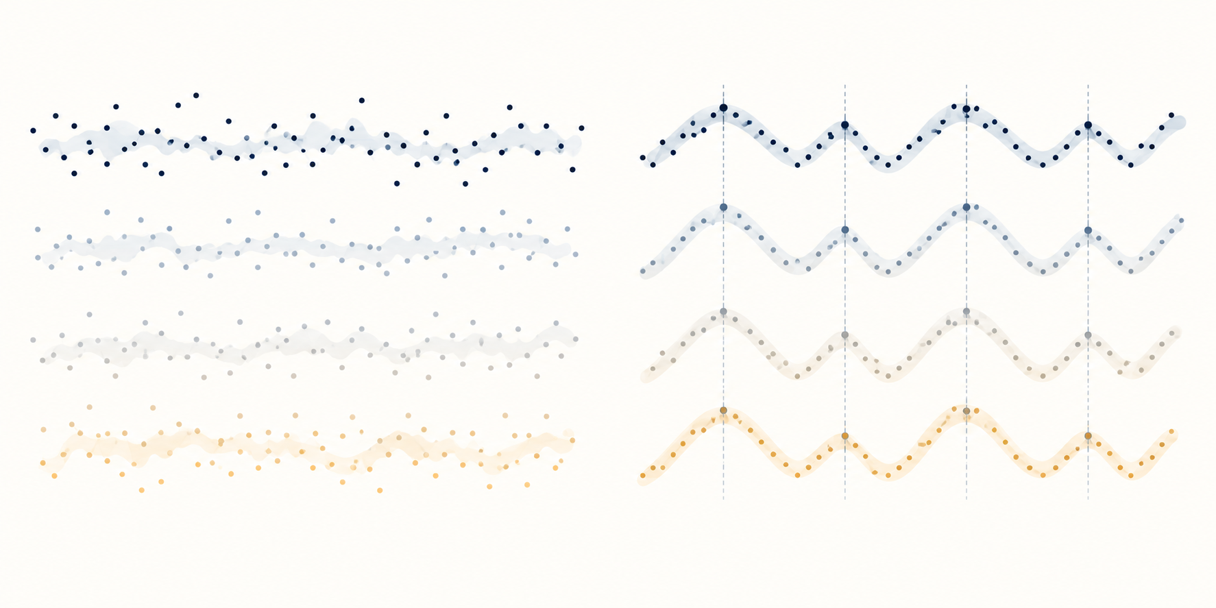
*वैचारिक चित्र बिना स्पष्ट lag pattern वाले residuals की तुलना कई offsets पर बार-बार संरेखित residuals से करता है; यह वास्तविक market observation नहीं है।*

Signed returns पर test लगाने से पूछा जाता है कि lag \(h\) तक linear autocorrelation संयुक्त रूप से शून्य है या नहीं। Fitted residuals पर लगाने से पूछा जाता है कि चुने गए model ने ऐसी linear dependence छोड़ी है या नहीं। Rejection mean specification, timing, market calendar और residual plots जाँचने का कारण दे सकती है; यह नहीं बताती कि कौन-सा term छूटा है।

Observation की परिभाषा autocorrelation पैदा कर सकती है, भले underlying one-period returns uncorrelated हों। उदाहरण के लिए, पाँच-session rolling return और अगला पाँच-session rolling return चार daily returns साझा करते हैं। Overlap पड़ोसी observations को यांत्रिक रूप से जोड़ता है। ऐसे constructed series में zero autocorrelation reject होना सही हो सकता है, लेकिन यह नहीं दिखाता कि non-overlapping daily return predict किया जा सकता था।

बताएँ कि observations daily returns हैं, rolling multi-day returns हैं, या overlapping outcomes के model residuals। Session calendar, closing timestamps और overnight interval को आर्थिक प्रश्न के अनुरूप रखें। Overlapping horizons जरूरी हों तो उस construction के अनुकूल inference और reference distribution लें; इसे standalone trading edge का प्रमाण न मानें।

Signed returns में autocorrelation कम होने पर भी volatility clustering हो सकती है। Residuals का square लेना सवाल बदल देता है: squared या absolute standardized residuals की autocorrelation return के scale में dependence का संकेत दे सकती है। McLeod और Li ने ARMA fitting के बाद nonlinear dependence के diagnostic के रूप में squared-residual autocorrelations का अध्ययन किया। यह diagnostic है, किसी एक volatility model का प्रमाण नहीं। ARCH-LM guide ARCH-type dependence के लिए अधिक लक्षित test बताती है और GARCH guide conditional-variance modeling समझाती है।

Zero autocorrelation, independence से कमजोर शर्त है। जाँचे गए lags पर correlations शून्य हो सकते हैं, फिर भी nonlinear transformations, conditional variance, tails या regimes पर dependence बच सकती है। Ljung–Box statistic अकेले normality, stationarity, causal structure या execution costs के बाद return कमाने की संभावना नहीं बताता।

सरल chi-square approximation model, residual construction, sample size और parameter-estimation setup पर निर्भर करती है। यदि पहले ARMA model fit किया गया, तो residual autocorrelations अनुमानित quantities हैं, सीधे देखे गए innovations के correlations नहीं। आम degrees-of-freedom adjustment एक उपयोगी asymptotic convention है, हर specification के लिए exact finite-sample guarantee नहीं।

छोटा sample, बड़ा lag horizon, लगभग एक-दूसरे को काटते AR और MA roots, outliers, conditional heteroskedasticity, या fitted model family के बाहर serial dependence—इनसे approximation कम भरोसेमंद हो सकती है। Rejection गलत mean specification, data-quality समस्या या अनुपयुक्त reference distribution दर्शा सकती है। Non-rejection का कारण कम power या dependence से चूका lag choice हो सकता है।

Complex या nonstandard model के लिए fit से मेल खाने वाला reference distribution रखने वाला diagnostic लें, या उचित bootstrap में estimation step दोहराकर calibration जाँचें। Dependence या बदलता variance चिंता हो तो iid residual resampling अपने-आप valid नहीं होती। Resampling design बताएँ और model selection को final evaluation से अलग रखें।

Rejection के बाद autocorrelation function, जहाँ उपयोगी हो partial autocorrelation, residual timing और \(Q_{LB}\) में lag-wise contributions देखें। विचारें कि pattern थोड़े समय का है, seasonal है, छूटे mean term से आया है या squared residuals में केंद्रित है। Model change किसी उचित specification question पर आधारित हो और उस data पर जाँचा जाए जिसका उपयोग उसे चुनने में नहीं हुआ।

Trading rule में sample pattern predict होना executable edge नहीं है। अगला forecast order से पहले उपलब्ध होना चाहिए, chronological holdout में टिकना चाहिए और bid–ask spread, market impact, commissions, funding, borrow और turnover को ध्यान में रखना चाहिए। Ljung–Box test strategy की net profitability नहीं जाँचता और rejection के out-of-sample बने रहने का प्रमाण नहीं देता।

Report में observation की परिभाषा और संख्या, tested series, transformations, lag limit, individual autocorrelations या plot, test variant, reference degrees of freedom, statistic, p-value और significance level दें। Financial returns में trading sessions, missing values, overlapping horizons और fitted conditional variance को कैसे संभाला, यह भी बताएँ। इससे पाठक समझ सकता है कि test ने क्या किया और क्या अनसुलझा छोड़ा।

Box और Pierce का 1970 paper overall residual-autocorrelation statistic विकसित करता है। Ljung और Box का 1978 paper finite-sample modification देता है। McLeod और Li का 1983 paper squared-residual autocorrelations देखता है। NIST Box–Ljung reference statistic और residual degrees-of-freedom adjustment बताता है। संबंधित diagnostics के लिए variance-ratio test, ARCH-LM और GARCH volatility clustering guides देखें।