

MIDAS Regression Explained: Mixed-Frequency Data and Volatility Forecasting
Learn how MIDAS regression combines daily and weekly financial data with parsimonious lag weights, how to build a volatility forecast, and where mixed-frequency models can mislead.
In this guideMIDAS addresses a mismatch in observation frequency
Short summary
MIDAS (mixed data sampling) regression connects observations recorded at different frequencies without first forcing every series onto one calendar. A small number of estimated parameters shape a weighted history of higher-frequency observations, which can help forecast a lower-frequency financial target. The weights describe a predictive pattern under a chosen model; they do not establish causation or a trading edge.
MIDAS addresses a mismatch in observation frequency
Financial and economic data do not arrive on one shared clock. A volatility target may be measured weekly, while its candidate predictors are daily returns or intraday realized measures. A macroeconomic series may be quarterly, while an asset price is observed every trading day. Ordinary regression expects the target and predictors to have one row per observation, so the analyst must decide what to do with these different calendars before estimating a familiar model.
One option is to aggregate daily inputs into a weekly average or sum. That is simple, but it forces a particular weight on each day and may discard where within the week a movement occurred. Another option is to repeat a quarterly value across daily rows or interpolate it. Repetition can make a slow-moving number look like many new observations; interpolation can introduce a smooth path that was never observed. Neither operation creates new information.
MIDAS gives a direct way to connect the frequencies. It keeps the target at its natural lower frequency and includes a structured lag of the higher-frequency series. The name refers to mixed data sampling, not to a single volatility model. Researchers use MIDAS regressions for volatility forecasting and for other settings where predictors have a finer sampling interval than the outcome. The central question is how much of the recent high-frequency history to use and how to constrain its weights.
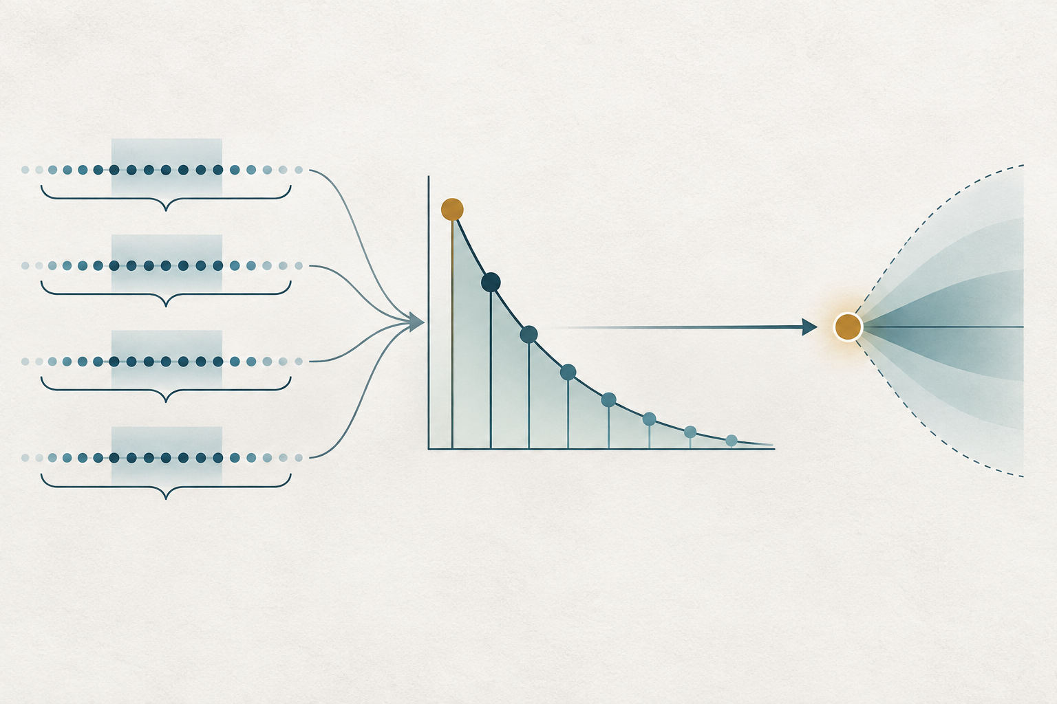
A weighted lag turns many observations into a compact predictor
Let \(y_{t+1}\) be a lower-frequency target, such as next week's realized variance, observed after week \(t+1\) ends. Let \(x_{t-j}\) be a daily predictor observed \(j\) trading sessions before the forecast origin at the end of week \(t\). A simple MIDAS regression is \(y_{t+1}=a+b\sum_{j=1}^{K}w_j(\theta)x_{t-j}+u_{t+1}\), where \(K\) is the number of daily lags, \(w_j(\theta)\) is a weight controlled by a small parameter vector, and \(u_{t+1}\) is the forecast error.
The weights are commonly normalized so that \(\sum_{j=1}^{K}w_j(\theta)=1\). This makes the weighted sum easier to read as a weighted history, while \(b\) controls how strongly that summary relates to the target. The normalization does not mean the daily observations are independent or equally informative. It is a convenient parameterization of the lag profile.
The analyst can choose \(x\) to be daily squared returns, absolute returns, a realized-variance measure built from intraday returns, or another variable available at the forecast origin. The outcome \(y\) might be a future weekly variance, a monthly macroeconomic release, or a different lower-frequency target. The target definition determines what the coefficients mean. A model for a realized-variance proxy is not automatically a model for latent instantaneous variance, option-implied variance, or a price return.
MIDAS is a regression framework rather than a universal estimator. The response can be modeled in levels, logs, or through a link function, and estimation depends on the chosen weight family and error assumptions. A linear regression of a nonnegative variance proxy can produce negative fitted values unless the specification constrains the forecast or transforms the target. The model's convenience does not remove the need to check the support and units of its target.
The weight function trades flexibility for stability
An unrestricted distributed-lag regression estimates a separate coefficient for each of the \(K\) daily inputs. If \(K\) is large relative to the number of weekly target observations, estimates can be noisy and strongly correlated. MIDAS instead defines the lag coefficients through a low-dimensional function. One illustrative exponential-Almon profile is \(w_j(\theta)=\frac{\exp(\theta_1j+\theta_2j^2)}{\sum_{\ell=1}^{K}\exp(\theta_1\ell+\theta_2\ell^2)}\). A normalized Beta-polynomial profile is another common choice.
These profiles can put more weight on recent sessions, taper gradually, or place relatively more weight on a middle part of the lag window. The parameters describe the chosen smooth curve, not the importance of each day without qualification. If the data support a short-lived response but the selected function forces a long smooth tail, the fitted coefficients inherit that restriction. Conversely, estimating many free daily coefficients may fit noise rather than stable dynamics.
Weight restrictions are modeling assumptions. Nonnegative normalized weights can make a variance forecast interpretable as a weighted average, but they rule out offsetting positive and negative lag effects. A flexible profile can allow a hump or changing slope, but too many shape parameters may be weakly identified. Researchers should compare a small set of defensible profiles, state which lags were available, and assess whether the forecast changes materially when the weight family changes.
There is no universal \(K\). A longer window may capture persistent information but adds parameters or forces a longer-shaped profile; a short window can miss slower dynamics. The lag count should be selected using information available in the estimation period and validated without using the future evaluation target. A good in-sample fit alone cannot decide whether the lag window captures a repeatable signal.
Align the forecast origin with when each value was knowable
Frequency labels are not enough to establish a valid forecasting design. Suppose the target is variance during the coming five-session week, and the forecast is issued after Friday's close. Predictors may include daily observations ending on that Friday, but not a realized-variance statistic computed from the coming week. If the target is a published weekly or monthly statistic, the publication timestamp can be later than the period it describes. A backtest must use the value as it was actually available, not the revised or subsequently published value.
Write down a forecast-origin table before fitting the model: the time the forecast is made, the latest permitted timestamp for each predictor, the target period, and the time the target becomes observable. For financial returns, specify whether the close-to-close return includes an overnight interval, which market session defines a day, and how holidays or missing bars change the count of daily lags. Five trading sessions and seven calendar days are different intervals.
Release calendars create ragged edges. At a given date, one predictor may have a fresh daily value while another monthly series has not yet been released. Carrying the last available monthly value forward can be valid if the model treats it as stale information known at the origin. It is invalid to fill in the not-yet-published observation using a later release. Historical revisions can create a subtler look-ahead problem: a current database may contain a revised macro series that a live forecaster could not have seen.
Asynchronous markets add another alignment issue. A daily equity close and a daily crypto close may refer to different UTC intervals; an intraday volatility estimate may use bars that complete after the forecast time. Time-zone conversion, daylight-saving changes, venue closures, and bar construction are part of the information set. State how these are handled rather than assuming that rows with the same date share the same information cutoff.
A hypothetical example converts daily inputs into a weekly forecast
Suppose the target is next week's realized variance, and the forecast is issued at Friday's close. The model uses five daily realized-variance inputs from the completed week. The estimated weights from most recent to oldest are \(0.40, 0.25, 0.16, 0.11, 0.08\), which sum to one. Suppose the corresponding daily inputs, in squared-return units, are \(0.0004, 0.0001, 0.0009, 0.0004, 0.0001\).
Their weighted history is \(0.40(0.0004)+0.25(0.0001)+0.16(0.0009)+0.11(0.0004)+0.08(0.0001)=0.000381\). For this hypothetical fitted model, let the intercept be \(a=0.00012\) and the slope be \(b=0.80\). The next-week variance forecast is \(0.00012+0.80(0.000381)=0.0004248\). If a standard-deviation summary is useful, its square root is about \(0.02061\), or \(2.06\%\) over the target week under the chosen target definition.
The arithmetic illustrates the mapping from daily predictors to a future weekly target; the values and fitted coefficients are invented. It does not say that any listed day caused next week's variance or that the asset is likely to rise or fall. The weight on the recent session says how the specified predictive model combines observed inputs, conditional on the sample and restrictions. It is not a causal response estimate.
The example also exposes a units question. Daily realized variance and weekly realized variance are both variances of returns, but they refer to different accumulation intervals. The slope \(b\), intercept, and target construction are learned for that exact convention; the daily inputs cannot simply be re-labeled as weekly variance. If the target were log weekly variance, the model's output would be in log units and exponentiating its conditional mean would generally not equal the conditional mean variance. Any transformation back to levels needs an explicit prediction target and, where appropriate, a retransformation correction.
Estimation depends on the target and the lag restriction
Given a fixed weight vector, the regression is linear in its intercept and slope. When the weights depend on unknown nonlinear parameters \(\theta\), estimation often uses nonlinear least squares or a related likelihood-based method. An estimator searches over the weight-shape parameters and regression coefficients together, or profiles out the linear coefficients for each candidate shape. Starting values, parameter bounds, convergence criteria, and the number of local optima can matter; a reported estimate should not hide failed or boundary solutions.
If \(y\) is a nonnegative volatility measure, an ordinary linear specification may generate a negative fitted value, especially out of sample. Options include restrictions that make the fitted level nonnegative, a positive link, or a model for the log of the target. These choices change the estimand and forecast interpretation. For a log-target model, a forecast of the conditional mean of log variance is not automatically the conditional mean of variance; the disturbance distribution and retransformation matter.
Sampling uncertainty also reflects how the target was constructed. Weekly realized variance from intraday returns is measured with error and can be sensitive to microstructure noise, sampling interval, jumps, and missing observations. If weekly target windows overlap, forecast errors from neighboring origins share underlying returns. Standard errors and comparisons that assume independent forecast errors may then be inappropriate. Use inference that matches the forecast horizon and dependence structure, and report the target's measurement procedure.
Parameter stability is another concern. An estimated weight profile averages across the estimation sample; if market structure changes, the curve can describe no current regime well. Expanding and rolling estimates answer different questions: the first uses more history but retains older dynamics, while the second adapts faster but has fewer observations and greater estimation noise. Prespecify the update rule and compare it to a fixed benchmark in chronological evaluation.
MIDAS is related to, but not identical to, GARCH-MIDAS
The word MIDAS names a way to combine differently sampled observations through weighted lags. A MIDAS regression can directly forecast a realized-volatility target from past daily or intraday measures. It does not have to specify the one-step conditional-variance recursion associated with a GARCH model.
GARCH-MIDAS is a distinct family that combines a slow-moving long-run volatility component, often driven by lower-frequency variables, with a short-run conditional-variance component that evolves recursively. The two components have their own parameterization and assumptions. A paper or software package using the label GARCH-MIDAS should be read through its exact equations: MIDAS weights may govern a long-run component while a GARCH recursion handles short-run shocks. The label alone does not reveal the target, whether the forecast is latent or realized volatility, or how positivity is enforced.
The original financial MIDAS volatility work compares different predictors, frequencies, and lag lengths in a parsimonious forecasting framework. Later methodological work develops estimation and testing properties for mixed-frequency regression models, including comparisons with traditional temporal aggregation. Those contributions support the mechanics, not a claim that MIDAS always outperforms GARCH or that high-frequency predictors always improve a forecast. Results depend on the asset, sample, target, predictor, horizon, and evaluation design.
Choose the model by the question. If the goal is to forecast a future realized-volatility measure using daily history, a direct MIDAS regression can be a natural candidate. If the goal is to model conditional variance recursively, compare an appropriate GARCH specification. If the task is to combine quarterly macro releases with a daily financial target, a mixed-frequency regression may need release-vintage controls. Models with similar names can answer different questions, so compare their forecast origins, target definitions, and information sets before comparing performance.
Measurement error and selection can overwhelm the weight curve
High-frequency data can improve temporal detail while worsening measurement noise. Very short bars contain bid–ask bounce, price discreteness, stale quotes, asynchronous trading, and feed errors. Summing squared returns at ever-shorter intervals does not guarantee a better realized-variance estimate. The sampling grid and cleaning rules should be chosen before examining forecast performance, with a sensitivity analysis for plausible alternatives.
The number of lower-frequency outcomes, not the apparent count of daily predictor rows, limits how much can be learned. A decade of daily inputs paired with weekly targets still provides only about five hundred weekly outcome periods before missing values and holdout evaluation. A smooth weight function uses fewer coefficients than a free daily lag, but its shape can still be weakly identified when the sample is short, predictors are highly persistent, or candidate lags are redundant.
Many analytical choices create selection bias: testing several high-frequency measures, lag lengths, weight profiles, transformations, markets, forecast horizons, and evaluation losses, then reporting only the best result. In-sample fit is especially vulnerable because the same targets guide the parameter and model choices. Preserve the tried model family, decide on a primary metric, and use a later chronological holdout or a selection-aware comparison. If many forecasts are compared on common dates, account for dependence and multiplicity rather than treating every result as an independent confirmation.
A fitted weight curve is not a causal explanation. High-frequency inputs can proxy for news, liquidity, or market activity; unobserved factors can drive both predictors and future volatility. Predictive usefulness requires stable timing and out-of-sample evidence. A causal interpretation would need a separate identification design and assumptions beyond the MIDAS lag equation.
A forecast does not define a profitable trading decision
A volatility forecast can inform a risk budget, hedge size, or scenario range, but it does not specify the sign of a return or the direction of a position. A predicted weekly standard deviation of \(2.06\%\) is not a promised move, a maximum loss, or an option-implied volatility quote. The forecast says something about a chosen dispersion measure under a fitted model and sample; realized returns can still be much larger or smaller.
For a strategy study, define the signal time, order time, instrument, exposure rule, and exit before testing. Re-estimate MIDAS parameters only with information that would have been available at each historical origin. Evaluate forecasts against a prespecified benchmark and a target-consistent loss, then separately simulate returns after spread, fees, funding, borrow, market impact, and turnover. A variance forecast can be statistically better while producing no improvement in after-cost returns.
Report the target and its sampling procedure; predictor definitions and units; lower and higher frequencies; forecast origin; lag count; weight function and constraints; estimation window and update schedule; handling of missing data and data vintages; loss function; benchmark; and chronological test dates. Show forecast uncertainty or sensitivity to the lag profile when those choices materially affect the result. For related background, see the guides to realized volatility, volatility clustering and GARCH, and forecast-accuracy comparisons.
The primary sources are Ghysels, Santa-Clara, and Valkanov's MIDAS volatility forecasting study, Ghysels, Sinko, and Valkanov's methodological review and extensions, and Andreou, Ghysels, and Kourtellos's analysis of mixed-frequency regression models. Their empirical results are tied to the samples and designs studied; they are not a guarantee of performance in a current market or another asset class.
Common questions
Q1Does MIDAS mean that all data are averaged to one frequency?
No. A MIDAS regression keeps the target at its chosen frequency and uses a structured weighted lag of higher-frequency predictors. It does not need to interpolate every series onto one common row-by-row calendar.
Q2Is MIDAS regression the same as GARCH-MIDAS?
No. MIDAS is a mixed-frequency weighted-lag framework. GARCH-MIDAS combines a MIDAS-style long-run component with a short-run GARCH variance recursion. Read the model equations to identify the target and components.
Q3Can a better MIDAS volatility forecast be used as a trading signal?
Not by itself. A volatility forecast describes a selected measure of dispersion. A strategy needs a separately specified directional or risk rule, realistic execution costs, and a chronological after-cost evaluation.
Sources and further reading
Report an issue
We’ll prepare an email with this article link. Mark receives the report only after you send it
Quick check
Read the guide? Check yourself with 3 questions
Question 01
What is the main role of the MIDAS weight function?
Choose an answer to see the explanation
Options glossary
A time-series model that updates conditional variance from past squared shocks and prior variance; it models volatility persistence, not return direction.
Read the deeper guideRealized volatilityVolatility calculated from price changes that occurred under a stated return, sampling-window, and annualization rule; different conventions can produce different values.
Read the deeper guideCausationA relationship describing how an outcome would differ under a specified intervention or counterfactual change; observed association alone does not identify it.
Read the deeper guide