Diebold–Mariano Test: How to Compare Forecast Accuracy

Suppose two models forecast the same return, volatility, or economic quantity over the same dates. Model A has a smaller average error than Model B in the evaluation sample. That describes the sample, but it does not tell you whether A is reliably more accurate or whether the observed gap could reflect ordinary variation in which dates happened to be tested.

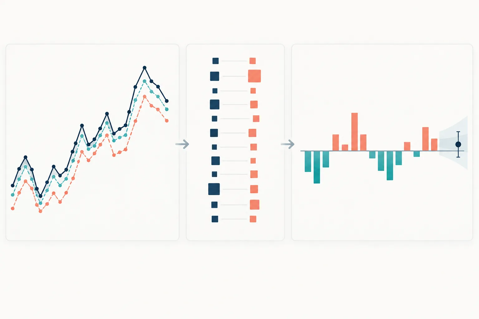
The Diebold–Mariano (DM) test turns that comparison into a paired time series. At each forecast origin, it compares the two forecasts against the same realized outcome, scores them using a loss function chosen in advance, and studies the sequence of loss differences. The pairing matters: a volatile market day can raise both models’ losses, while the comparison asks whether one model tends to lose less on those very same days.

The original framework is not limited to squared error or normally distributed forecast errors. It can compare different loss functions, including asymmetric ones, when those scores match the forecast question. It does require a defensible evaluation design and an estimate of the uncertainty in the average loss difference. Diebold and Mariano (1995) set out the equal predictive accuracy test; Harvey, Leybourne, and Newbold (1997)00719-4) study a small-sample modification.

Each row should represent a comparable forecast origin. Both models need to predict the same target, for the same horizon, from information that was available at that origin. Align the realized outcomes, time stamps, currency or unit, data vintage, and missing-observation rules before comparing losses. If one model predicts tomorrow’s close and the other predicts a five-day average, their errors answer different questions.

Use predictions generated without looking ahead. A chronological holdout or rolling pseudo-out-of-sample design can do this, but a split alone is not enough if the same holdout was repeatedly used to tune features, thresholds, or model variants. Preserve the forecast made at each historical origin, including the data and model version that produced it. Revised macroeconomic data, survivorship filters, or future corporate-action adjustments can otherwise change the evaluation after the fact.

The two models should be evaluated on the same set of origins. Dropping difficult dates for one model but not the other breaks the paired comparison. If forecasts are missing, define a common sample or give a justified treatment of missing predictions; do not quietly let the models face different market regimes. Choose the start and end dates before examining which sample produces the preferred result.

Let the realized value at origin t be yₜ and the model forecasts be ŷA,ₜ and ŷB,ₜ. Their errors are eA,ₜ = yₜ − ŷA,ₜ and eB,ₜ = yₜ − ŷB,ₜ. A loss function L turns each error into a score where lower is better. Squared-error loss, L(e) = e², penalizes large misses more heavily. Absolute-error loss, L(e) = |e|, grows linearly with the miss. A quantile forecast may instead use an asymmetric pinball loss because under- and over-predicting have different costs.

The chosen score can change which model appears better. Consider two hypothetical error pairs measured in the same units: Model A has errors 0 and 2; Model B has errors 1 and 1. Under squared loss, their average losses are 2 and 1, so B scores better. Under absolute loss, both average losses are 1. Neither calculation is universally correct: each answers a different question about the errors that matter.

For return forecasts, squared error may be useful for a conditional-mean forecast, while a volatility forecast needs a score designed for the target, and a Value-at-Risk forecast needs a quantile score or a risk-specific backtest. Selecting the loss after seeing which model wins turns the test into another search. Write down the loss and the direction of “better” before examining the comparison.

A VaR forecast targets a tail quantile rather than an ordinary point forecast. The VaR backtesting guide explains how exception-frequency and timing tests evaluate that separate risk forecast.

For a lower-is-better loss, define the period-t difference as

dₜ = L(eA,ₜ) − L(eB,ₜ)

With this sign convention, a positive dₜ means Model B had the lower loss on that origin; a negative value favors Model A. The sample average is d̄ = (1/n) Σ dₜ. The unconditional equal-accuracy null is E[dₜ] = 0. A two-sided alternative asks whether expected losses differ in either direction. A pre-specified one-sided alternative can ask whether one named model has lower expected loss.

The basic statistic is

DM = d̄ / √(Ŝd / n)

Here Ŝd estimates the long-run variance of the loss-difference series, not just the variance of either model’s forecast errors. Under the null and appropriate regularity conditions, the statistic is asymptotically standard normal. Large positive values favor B under the sign convention above; large negative values favor A. The p-value measures compatibility with the specified null and sampling assumptions, not the probability that either model is true.

Pairing removes irrelevant differences in the two models’ overall error scales only to the extent captured by their per-origin differences. It does not make the loss series independent, remove parameter-estimation uncertainty automatically, or correct a search over many targets and specifications. Those choices belong in the design and uncertainty calculation.

Suppose 100 matched, hypothetical one-step forecasts have mean squared loss of 0.26 for Model A and 0.23 for Model B, in squared percentage-point units. The average difference is therefore d̄ = 0.26 − 0.23 = 0.03, which favors B. For this deliberately simple example, assume the estimated long-run variance of dₜ is 0.04 and there is no serial covariance across origins.

The estimated standard error of the average difference is √(0.04 / 100) = 0.02. The unadjusted statistic is 0.03 / 0.02 = 1.50. For horizon h = 1 and T = 100, the Harvey–Leybourne–Newbold small-sample factor is √[(T + 1 − 2h + h(h − 1)/T) / T] = √0.99 ≈ 0.995. Multiplying gives an adjusted statistic near 1.49; using the approximate t₉₉ reference distribution gives a two-sided p-value of about 0.14.

B has the lower observed mean squared error, but this example does not provide strong evidence against equal expected accuracy at conventional significance thresholds. A non-rejection does not prove that the models are equally accurate; a rejection would still be conditional on the chosen score, origins, and assumptions. The variance value and all losses here are hypothetical teaching inputs, not empirical results.

The corresponding root mean squared errors are about 0.510 and 0.480 percentage points, a descriptive gap of 0.030. The DM statistic still uses paired squared-loss differences; it is not a t-test of the two square roots.

If five-day-ahead forecasts are issued every day, adjacent forecasts share four of their five target days. Their errors, losses, and loss differences can therefore move together. Treating 100 daily forecast origins as 100 independent comparisons can understate uncertainty and make the statistic look too large.

The long-run variance accounts for serial covariance in dₜ. A common heteroskedasticity-and-autocorrelation-consistent estimate has the form

Ŝd = γ̂₀ + 2 Σₖ₌₁ᵐ wₖ γ̂ₖ

where γ̂ₖ is the sample autocovariance of d at lag k, wₖ is a kernel weight, and m is the selected bandwidth. Newey and West (1987) give a positive semi-definite HAC covariance estimator. For ideal h-step forecast errors under the relevant assumptions, overlap often induces dependence through at least h − 1 lags; the original DM setup discusses a truncated estimate for that case. Real data may have longer dependence from persistent targets, rolling estimation, or strategy construction, so h − 1 is not a universal bandwidth rule.

State the horizon, kernel, bandwidth, and any small-sample adjustment. Show whether conclusions change under reasonable dependence settings rather than choosing a bandwidth because it gives a preferred p-value. If evaluation origins are spaced far enough apart to avoid overlap, say so and explain what information or sample size that choice sacrifices. Dependence-aware uncertainty is part of the test, not an optional display setting.

The usual DM comparison is easiest to interpret for forecasts that are not nested under the equal-accuracy null. If a larger model contains a smaller benchmark, the additional estimated coefficients can add forecast noise even when their true values are zero. Under that null, the ordinary difference in mean squared errors can have a nonstandard distribution. For nested-model MSPE comparisons, a method such as the Clark–West adjustment accounts for this estimation-noise effect; it is not a general replacement for DM in every model design. See Clark and West (2007).

The ordinary DM null concerns average, unconditional loss across the evaluation sample. It can hide changes over time: A may do better in calm periods and B during volatile periods while their overall means are similar. If the question is whether relative accuracy depends on information known at the forecast date, conditional predictive ability tests use loss differences together with pre-specified instruments. Giacomini and White (2006) develop such a framework. Its assumptions and evaluation-window design matter, so adding arbitrary indicators after inspecting results is not a valid shortcut.

A test choice should follow the comparison structure: independent forecasts, nested models, changing conditional skill, or a family selected from many candidates are not interchangeable cases. For the last case, White’s Reality Check and Hansen’s SPA guide explains family-wide correction after searching many trading rules.

A forecast can be statistically more accurate yet fail to improve net trading results. A strategy must map the forecast into a position, choose when to trade, and bear spreads, commissions, slippage, market impact, funding, borrow, and risk limits. A tiny improvement in average squared return error may have no useful effect on decisions, while a model with slightly worse average error may better identify a tail event that matters to a particular rule.

Keep forecast evaluation and portfolio evaluation as separate steps. First test the forecast against a target and loss that match the stated prediction task. Then evaluate a fully specified trading rule on data that did not select the forecast, with realistic execution and financing assumptions. A forecast-test p-value is not a backtest return, a Sharpe ratio, or a probability of future profit.

Repeatedly trying models, targets, horizons, loss functions, and sample windows creates selection bias even if each individual DM calculation is correct. Record the full search and use a family-wise method when the research question is whether any candidate survived that search. The block-bootstrap guide covers dependence-preserving uncertainty for a preselected statistic; it does not by itself correct selection from an undocumented model search.

Name both forecast models, the benchmark relationship, the target, horizon, forecast-origin schedule, evaluation dates, information set, data vintage, and common-sample rule. Define the loss mathematically and state whether positive dₜ favors A or B. Report n, the average loss of each model, d̄, the long-run variance estimator, HAC kernel and bandwidth, small-sample correction, reference distribution, test direction, and p-value.

Also state whether models are nested, how parameters were estimated, whether the comparison was chosen before or after inspecting results, and which other variants were tried. If the sample was used for model selection, label the test as such rather than calling it untouched out-of-sample evidence. A clean report lets readers see exactly what the test compares and which uncertainty or selection problems remain outside it.