VaR Backtesting: Kupiec and Christoffersen Tests Explained

Value at Risk (VaR) is a loss threshold tied to a confidence level and horizon. If a one-day 99% VaR forecast is $10,000, the model assigns a 1% probability to a one-day loss worse than $10,000, under the model’s stated information and assumptions. VaR does not cap the loss at $10,000, and it does not describe how large a loss could be after that threshold is crossed.

Backtesting turns a sequence of forecasts and outcomes into a sequence of exceptions. With a 99% one-day VaR, a well-calibrated model should produce exceptions about 1% of the time over repeated comparable observations. This statement has two parts: the long-run frequency should be near the target, and the exceptions should not arrive in a pattern that contradicts the model’s conditional risk forecasts. The Kupiec proportion-of-failures (POF) test focuses on the first part. Christoffersen’s independence and conditional-coverage tests bring the order of exceptions into the analysis.

The distinction is practical. A model can have four exceptions in a year and still place all four next to one another during a turbulent week. Another model can have four exceptions spread across the year. A count-only test sees four in both cases. A timing test sees different hit sequences. The tests below help describe those features; they do not replace review of the underlying positions, market data, assumptions, or loss severity. A separate guide explains how [GARCH models represent volatility clustering](/en/learn/volatility-clustering-garch-explained); a variance model and a backtest answer different questions.

Use one sign convention throughout. Let Lₜ be the realized loss on day t and VaRₜ|ₜ₋₁ the one-day threshold forecast with information available before day t. Define the exception indicator as Iₜ = 1 when Lₜ > VaRₜ|ₜ₋₁, and Iₜ = 0 otherwise. If the model is a 99% VaR model, the target exception probability is α = 1 − 0.99 = 0.01. Some sources define the indicator using returns or define a covered interval instead; those conventions are equivalent after translating the sign and probability. State which one is being used.

The forecast and outcome must refer to the same portfolio, horizon, valuation time, and loss definition. For a forecast made after the close for the next trading day, compare it with that next day’s loss under a consistently specified valuation rule. Decide in advance how to treat equality at the VaR boundary, holidays, missing observations, market closures, intraday corrections, and any portfolio changes. These choices can change the hit sequence, especially when breaches are rare.

Keep model fitting separate from final evaluation. If parameters or risk thresholds were chosen after reviewing the same period used for the test, the resulting p-value no longer describes a clean out-of-sample check. For rolling forecasts, record when each forecast was produced and which information was available then. Overlapping multi-day forecasts can create dependence in the exception sequence even if one-day exceptions would have been independent. The standard tests below should not be treated as automatic fixes for mismatched horizons, look-ahead, revised inputs, or a model-selection process.

Suppose there are T comparable forecast-outcome pairs and x exceptions. The observed exception rate is p̂ = x/T. Kupiec’s proportion-of-failures test, also described as an unconditional-coverage test, compares two binomial likelihoods: one fixes the exception probability at the target α, and the other estimates it freely as p̂. The test originates in Kupiec’s 1995 paper, with a Federal Reserve archive record. Its likelihood-ratio statistic is

LRᵤ꜀ = −2 ln [ (1−α)^(T−x) α^x / ((1−p̂)^(T−x) p̂^x) ].

Under the null that exceptions are independent Bernoulli events with probability α, the statistic is approximately chi-square with one degree of freedom in a sufficiently large sample. A large statistic rejects the specified exception frequency. Because the alternative uses the observed rate freely, the test can reject when the model produces too many exceptions or too few. A model that almost never breaches its VaR is not automatically calibrated: it may be so conservative that its risk forecasts are not useful for their intended purpose.

The POF test uses the count x, not the dates on which exceptions occurred. Permuting the same hit indicators leaves its statistic unchanged. So a POF result cannot tell whether four exceptions were spread out or consecutive. The Bernoulli likelihood also assumes the exception indicators are independent for its reference distribution. When the question is whether exceptions are clustered, add a test designed for dependence rather than reading clustering into the POF result.

Consider a hypothetical series of 250 one-day forecasts at 99% VaR. The target rate is α = 0.01, so the expected exception count under the null is Tα = 250 × 0.01 = 2.5. Suppose the series contains four exceptions. The observed rate is p̂ = 4/250 = 0.016, or 1.6%. That is above the 1% target, but the gap alone does not determine whether the likelihood-ratio test rejects.

Substituting T = 250, x = 4, and α = 0.01 gives LRᵤ꜀ ≈ 0.769. Using the asymptotic chi-square(1) reference gives p ≈ 0.38; the 5% critical value is about 3.84. Under that approximation, this example does not reject unconditional coverage at the 5% level. The calculation is hypothetical, not an empirical result or a recommended acceptance threshold.

The two log-likelihoods show where the statistic comes from. With the target rate fixed, ℓ₀ = 246 ln(0.99) + 4 ln(0.01) ≈ −20.893. At the unrestricted observed rate, ℓ₁ = 246 ln(0.984) + 4 ln(0.016) ≈ −20.508. The unrestricted fit is higher by about 0.385 log-likelihood units, so LRᵤ꜀ = −2(ℓ₀ − ℓ₁) ≈ 0.769. The test measures this loss of fit relative to the target-rate model; it is not a distance in dollars.

The non-rejection does not establish that the model is well calibrated. Only 2.5 exceptions were expected, so one or two additional events noticeably change the observed rate. The chi-square calculation is asymptotic, and rare-event tests can have limited power in samples of this size. Read the statistic together with the expected count, forecast horizon, test design, and sample size. A p-value is not the probability that the VaR model is true.

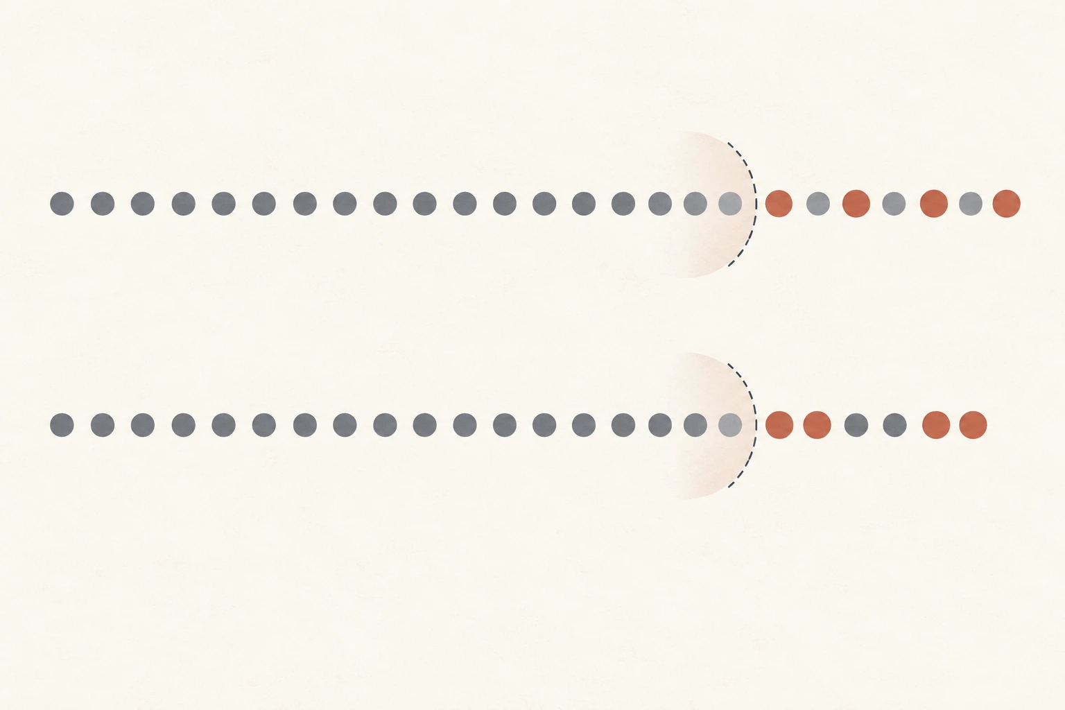
Now compare two hypothetical 250-day sequences, each with four exceptions. In sequence A, the exceptions occur on days 20, 80, 140, and 220. In sequence B, they occur on days 60, 61, 180, and 181. Both have x = 4 and p̂ = 1.6%, so their Kupiec statistic is identical. But B contains two adjacent exception pairs while A contains none.

The sketch below shows why it is useful to preserve the hit sequence instead of reporting only its total. It is conceptual, not a 250-day data series and not a test result. Consecutive exceptions can be consistent with a model that fails to respond to changing volatility, but a small number of points cannot diagnose the cause by itself. The pattern may reflect model misspecification, a market shock, portfolio changes, overlapping horizons, or data and timing conventions.

For the transition count, let nᵢⱼ be the number of times the previous indicator is i and the current indicator is j, with 0 meaning no exception and 1 meaning an exception. Away from sample boundaries, sequence A has n₀₁ = 4 and n₁₁ = 0, whereas B has n₀₁ = 2 and n₁₁ = 2. Both have four exceptions; the counts differ because some hits in B follow another hit. This is the information a first-order independence test uses.

Using the transition totals, the fitted probability of a hit after a non-hit is n₀₁/(n₀₀+n₀₁); after a hit it is n₁₁/(n₁₀+n₁₁). A has 4/245 ≈ 1.63% after a non-hit and 0/4 after a hit. B has 2/245 ≈ 0.82% after a non-hit and 2/4 = 50% after a hit. The 50% is based on only four transitions from a hit, so it is a property of this tiny hypothetical sequence, not a credible estimate of a real model’s next-day risk.

Christoffersen’s 1998 paper develops conditional interval-forecast evaluation. Its independence test compares the exception rate after a quiet day with the rate after an exception. Write π₀ = Pr(Iₜ = 1 | Iₜ₋₁ = 0) and π₁ = Pr(Iₜ = 1 | Iₜ₋₁ = 1). Under the independence null, π₀ = π₁: the previous day’s hit status does not change the probability of a hit today. Under the alternative, the two transition probabilities are estimated separately from n₀₀, n₀₁, n₁₀, and n₁₁.

The likelihood-ratio independence statistic compares those two models and is also commonly evaluated against a chi-square distribution with one degree of freedom. Unlike the POF test, it depends on the order of the indicators. If exceptions tend to follow exceptions, π₁ may exceed π₀. The test is specifically about first-order dependence in this binary sequence; it does not test every way that past information, volatility, or portfolio state could predict future losses.

With only a few exceptions, transition estimates can be especially unstable. A sequence with no consecutive hits may produce a boundary estimate of zero for π₁, but that does not show that a second hit is impossible. It only says that none occurred in this sample. Check transition counts and the sample size alongside the statistic. Avoid interpreting a sparse table as a precise estimate of next-day tail risk.

The conditional-coverage test combines the Kupiec frequency statistic with Christoffersen’s independence statistic: LR꜀꜀ = LRᵤ꜀ + LRᵢₙd. Its joint null is that the exception probability equals α and that exceptions are independent over time. Under the standard large-sample setup, the sum is compared with a chi-square distribution with two degrees of freedom.

Report the component results as well as the combined test. A rejection of conditional coverage means the joint requirements are inconsistent with the observed sequence under the test assumptions, but it does not identify the cause. If the POF test rejects and independence does not, the count may be the clearer signal. If the independence test rejects, exception timing deserves attention even when the total count looks close to target. If neither rejects, the sample may still be too short to reveal a misspecification.

The test has a narrow interpretation. It compresses each day to a binary outcome, so it does not measure whether a loss exceeded VaR by $1 or by $1 million. It also cannot validate the rest of the loss distribution or establish that Expected Shortfall is correct. For how VaR and Expected Shortfall answer different tail-risk questions, see the guide to [VaR versus Expected Shortfall](/en/learn/value-at-risk-vs-expected-shortfall-explained).

At 99% VaR, a 250-day sample has only 2.5 expected exceptions. Under independent 1% hits, the expected number of hit-to-hit transitions across 249 adjacent pairs is roughly 249 × 0.01² = 0.025. Most such samples will contain no adjacent pair even when the model is correctly calibrated. This scarcity makes it difficult to estimate the transition probabilities with precision and can leave a dependence test with little power.

Christoffersen and Pelletier report that existing VaR backtests can have relatively low power in realistic small samples and study duration-based tests that model the time between exceptions in their 2004 paper. Their results motivate an additional diagnostic; they do not make a duration test universally superior or remove the need to match the test to the risk forecast and sample design. When observations are few, say so instead of treating a non-rejection as a clean bill of health.

The target tail rate matters. At 95% VaR, the nominal rate is 5%, so a 250-day sample has 12.5 expected exceptions; at 99.9%, it has only 0.25. The same test statistic label does not guarantee comparable evidence across these designs. Explain the confidence level, horizon, number of observations, target and observed counts, transition counts, and whether the calculation is asymptotic or uses a finite-sample method.

Choose the next diagnostic by asking what information the two tests discarded. If you want to test whether exceptions are predictable from lagged hits, VaR forecasts, or other variables known at forecast time, Engle and Manganelli’s dynamic-quantile (DQ) test in their CAViaR paper tests restrictions on centered exception indicators and a chosen instrument set. Its conclusion depends on those instruments and their timing; it is not a test of every conceivable conditional failure. A duration-based test instead examines waiting times between exceptions. Each expands a different part of the analysis.

If the concern is loss severity beyond the VaR boundary, frequency and independence tests are not enough. Review the size of exceedances and choose an Expected Shortfall evaluation method suited to the forecast and assumptions. If the concern is selecting the strongest result after trying many models, VaR backtesting does not solve the strategy-selection problem; see [PBO and CSCV](/en/learn/probability-of-backtest-overfitting-cscv-explained) for a distinct rank-based diagnostic.

A useful report states the portfolio and loss convention, forecast horizon, confidence level, evaluation dates, how forecasts were generated, the exception definition, observed and expected counts, POF statistic, transition counts, independence and conditional-coverage results, and limitations from sample size or overlapping horizons. Pair the tests with plots of forecast thresholds and realized losses, and keep later evaluation data closed while choosing the model. These steps make the evidence interpretable; they do not turn a historical pass into a guarantee of future risk control.