

Probability of Backtest Overfitting (PBO) and CSCV Explained
Learn how combinatorially symmetric cross-validation estimates PBO, how out-of-sample ranks become logits, and why the statistic is not a forecast of future losses
In this guidePBO measures the selection process, not a strategy in isolation
Short summary
The probability of backtest overfitting (PBO) asks how often the strategy selected as best in-sample ranks below the candidate set’s median out-of-sample. Combinatorially symmetric cross-validation (CSCV) estimates that frequency by repeatedly assigning half of equal time blocks to selection and the other half to evaluation. PBO is a diagnostic of a specified search, score, and historical performance matrix; it is not the probability that a live strategy will lose money.
PBO measures the selection process, not a strategy in isolation
A research team may try different lookbacks, entry thresholds, holding periods, universes, cost assumptions, and portfolio constraints, then keep the variant with the highest backtest score. The selected result has benefited from every opportunity to fit the particular sample. PBO describes one consequence of that search: across a defined set of in-sample and out-of-sample partitions, how often does the in-sample winner land below the median of the same candidate set out-of-sample?
Bailey, Borwein, López de Prado, and Zhu introduced PBO as a framework for strategy-selection risk and proposed CSCV as one way to estimate it. Their definition concerns the selection procedure among tested configurations, not simply whether an individual forecasting equation has too many parameters. In their terminology, “in-sample” is the subset used to choose among candidate strategies for a split. It need not be the period used to estimate every underlying model. Read the original PBO paper for the formal setup.
That distinction matters in practice. A single strategy can have a high full-sample Sharpe ratio and still be the luckiest member of a weak research family. Conversely, a selection process can usually choose a candidate that ranks above its peers out-of-sample even if the entire group has negative returns. PBO compares ranks within the submitted candidate set; it does not by itself test whether a strategy has positive expected return.
PBO answers a different question from other validation tools
A chronological holdout or walk-forward test asks how a specified research process performed on later observations that were not used to make earlier decisions. Purged cross-validation addresses overlap between training labels and test outcomes; an embargo can add a separately justified buffer. Neither operation, by itself, measures how frequently the winner of a broad strategy search falls below the candidate median. For the mechanics of purging and embargo, see the guide to [purged cross-validation and embargo](/en/learn/purged-cross-validation-embargo-time-series-finance-explained).
PBO also differs from a multiple-testing adjustment. White’s Reality Check uses a bootstrap framework to test whether the best rule in a family outperforms a benchmark after accounting for data snooping. The Deflated Sharpe Ratio adjusts a Sharpe-based significance calculation for selection effects and non-normal returns. PBO instead summarizes the out-of-sample rank of the in-sample-selected candidate across a set of partitions. These methods use different statistics and assumptions, so one does not automatically substitute for the others. See White’s original Reality Check paper and Bailey and López de Prado’s Deflated Sharpe Ratio paper.
Start with a complete, synchronized performance matrix
Let M be a T × N matrix. Each of its N columns is one candidate strategy or configuration, and each of its T rows is the same observation interval across every candidate. A row might be a daily return after the costs that belong in the research claim. If candidates trade at different frequencies, first define a common time index and aggregate their performance consistently; comparing one strategy’s daily returns with another’s monthly totals would not create a meaningful row-by-row matrix.
The candidate set should reflect the actual selection opportunity: variants rejected by a grid search, manual changes made after seeing results, different universes, and alternative rules that contributed to the final choice. PBO can only assess the candidates and performance histories supplied to it. If a team logs only the finalists after a much larger search, the resulting estimate understates the search that actually occurred.
Use the same return convention, currency, leverage treatment, and performance criterion for every candidate. If selection uses net Sharpe, construct each column with the relevant fees, spread, financing, funding, borrow, and execution assumptions before computing that Sharpe. The metric must also be computable on the subsets used below. The original paper requires synchronized rows across candidates and a criterion that can be estimated on each subsample; when trade frequency differs, it recommends matching the series to a common index.
CSCV pairs every half-sample with its complement
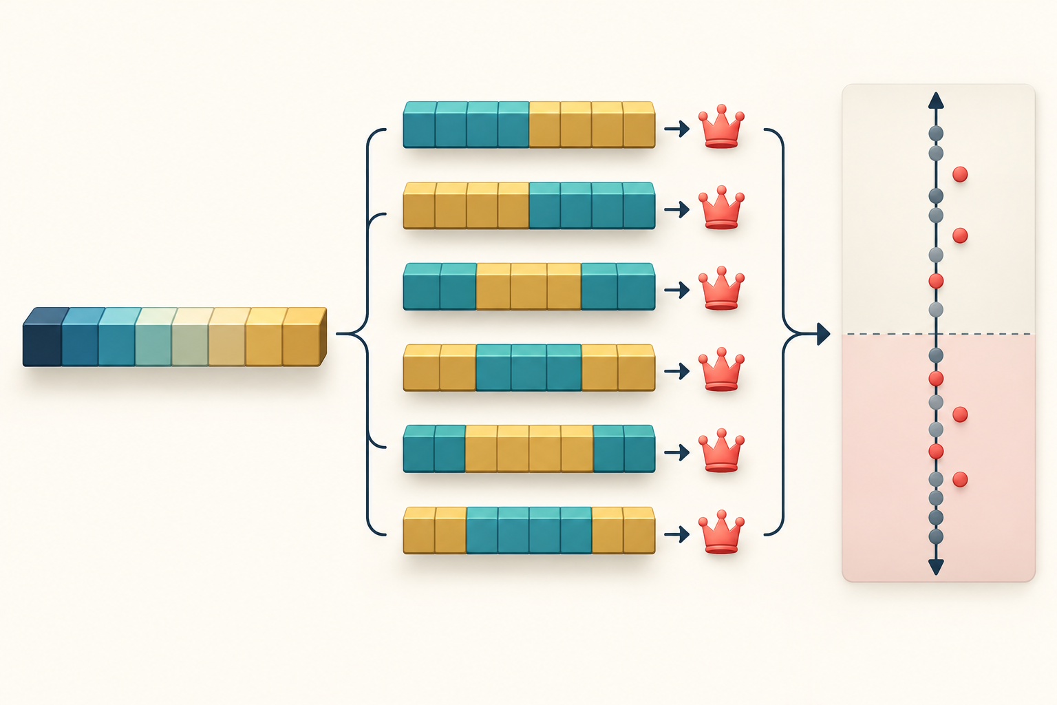
Choose an even number S of equal-sized, disjoint time blocks. Keep each block’s internal time order. For every possible choice of S/2 blocks, combine those blocks as the in-sample (IS) set and use the remaining S/2 blocks as the out-of-sample (OOS) set. Preserve the original order of the selected blocks when calculating a path-based statistic, and document what the joins mean for that metric.
The number of IS assignments is C(S, S/2). With four blocks A, B, C, and D, the six assignments are AB, AC, AD, BC, BD, and CD; each assignment’s complement also appears as its own assignment. With S = 16, the count is C(16, 8) = 12,870. These are deterministic combinations of the same history, not 12,870 independent market experiments.
“Symmetric” refers to reusing the complement as the selection set in another combination: for example, AB is IS and CD is OOS in one split, while CD is IS and AB is OOS in another. “Combinatorial” refers to enumerating all half-block choices rather than drawing one random split. The procedure is not a chronological replay. A selected set can include early and late blocks while its complement contains middle blocks, so CSCV’s OOS label does not mean “the future after the training period.”
Convert the selected candidate’s OOS rank to a logit
For split c, apply the research selection rule to the IS subset and choose the best candidate, denoted n*(c). Then score all N candidates on the complementary OOS subset using the same performance measure. Rank the selected candidate among those N OOS scores, defining rank r(c) so that 1 is worst and N is best. State how ties are handled and keep that convention fixed across splits.
Convert the rank to a relative rank ω(c) = r(c)/(N+1). Dividing by N+1 keeps the value strictly between zero and one, even for the lowest or highest rank. The logit is λ(c) = ln(ω(c)/(1−ω(c))). It is negative when the selected candidate ranks below the set’s median, zero at the median, and positive when it ranks above the median. The estimated PBO is the share of all CSCV assignments with λ(c) ≤ 0.
The scalar PBO reports how often the in-sample winner falls at or below the median OOS. The full logit distribution adds information: its center and left tail show whether selected candidates usually remain near the middle, often fall well below it, or tend to rank above it. A logit is a transformed relative rank, not a probability assigned to an individual live trade or a calibrated forecast of a future return.
A hypothetical four-block example gives PBO of 66.7%
Suppose a researcher has four equal historical blocks and four candidate rules, labeled R1 through R4. The six IS assignments are shown below. The “OOS rank” column is the rank of the rule selected in that row’s IS subset, among all four rules on the complementary blocks. Every value is hypothetical and is provided only to show the calculation; it is not a measured result or market observation.
| IS blocks | IS winner | OOS rank r | Relative rank ω = r/5 | Logit ln(ω/(1−ω)) | At or below median? |
|---|---|---|---|---|---|
| AB | R1 | 1 | 0.20 | −1.386 | Yes |
| AC | R3 | 4 | 0.80 | +1.386 | No |
| AD | R2 | 2 | 0.40 | −0.405 | Yes |
| BC | R1 | 1 | 0.20 | −1.386 | Yes |
| BD | R4 | 3 | 0.60 | +0.405 | No |
| CD | R3 | 2 | 0.40 | −0.405 | Yes |
Four of the six selected rules have an OOS relative rank no greater than one-half, so the empirical PBO is 4/6 ≈ 0.667, or about 66.7%. For example, rank 2 gives ω = 2/(4+1) = 0.4 and λ = ln(0.4/0.6) ≈ −0.405. Rank 3 gives ω = 0.6 and the opposite logit, about +0.405.
This example does not mean there is a 66.7% chance of losing money next month. It means that, in this hypothetical matrix and under this ranking convention, the IS winner fell at or below the candidate median in four of the six enumerated partitions. Even the remaining two winners could have negative absolute OOS returns while ranking above their peers.
Treat PBO as a conditional diagnostic with limits
PBO depends on the candidate family, the observed performance matrix, the selection metric, the time blocks, and the tie rule. Unrecorded experiments remain outside its scope. “Model-free” means the calculation can operate on candidates’ performance histories without knowing their forecasting equations; it does not mean the result is free from design choices, data quality, or assumptions.
CSCV combines blocks into symmetric subsets, which helps compare equal-sized IS and OOS samples. It also means the OOS set is generally not one later chronological interval. Recombining blocks can disrupt long-range dependence, seasonal structure, or economic regimes. The number S controls both the number of combinations and the duration represented by each block; choose it with the strategy’s relevant horizons and structure in mind, and report it. A large combination count does not create the same number of independent observations because the combinations reuse the same blocks.
The statistic inherits biases in the source returns. Survivorship, revised data, unavailable-at-the-time features, unrealistic fills, omitted costs, and a selected universe can all make every candidate history misleading. CSCV does not automatically purge overlapping label intervals, refit every model pipeline inside each split, or prevent information from leaking through preprocessing. Those steps must match the research question and be implemented explicitly. For chronological leakage protections, compare the official TimeSeriesSplit documentation and the purged-validation guide.
Path-dependent measures such as maximum drawdown need extra care: concatenating nonadjacent blocks changes the path and may change the statistic. The PBO paper notes that the order of observations matters for some measures even when it does not matter for Sharpe. Do not treat every performance metric as interchangeable in CSCV. Explain how order, gaps, missing observations, and compounding are handled before interpreting a rank.
Report PBO beside chronological evidence and the full search record
Before calculating PBO, preserve the candidate registry, every adjustment made after viewing results, the performance matrix, the selection metric, and the rule for ties. Report T, N, S, block construction, C(S,S/2), the OOS rank convention, the estimated PBO, and a view of the logit distribution. Also report absolute OOS performance, costs, turnover, drawdowns, and the number of candidates that lose; rank alone hides whether every candidate is weak.
Use a walk-forward or other genuine chronological holdout to answer how the frozen research process performs on later data. Keep that final period closed while choosing the model and thresholds; repeatedly checking it turns it into another selection set. Time-ordered tools such as TimeSeriesSplit implement chronological folds under their documented assumptions, while PBO measures a different rank-based property of the searched candidate family.
PBO can therefore complement, but not replace, label-overlap controls, multiple-testing analysis, realistic execution modeling, prospective evaluation, and live monitoring. To continue, see [multiple testing and false discovery in finance](/en/learn/multiple-testing-false-discovery-rate-finance-explained) and [Sharpe-ratio serial-correlation adjustments](/en/learn/sharpe-ratio-serial-correlation-annualization-explained). No single statistic turns a historical ranking into proof of a persistent trading edge.
Common questions
Q1Does PBO mean the strategy has that probability of losing money?
No. PBO estimates how often an in-sample-selected candidate ranks at or below the candidate median in the specified partitions. It is not a probability of a future loss or a calibrated live-return forecast.
Q2Is CSCV the same as walk-forward testing?
No. CSCV pairs every half-block selection set with its complement, so its OOS subset can contain earlier and later blocks. Walk-forward testing keeps training before each later test period to examine a chronological deployment-like path.
Q3Does a low PBO prove the selected strategy has an edge?
No. The winner can rank above a weak candidate set while still losing in absolute terms. Assess net returns, uncertainty, costs, leakage, and performance on genuinely later data as separate questions.
Sources and further reading
Report an issue
We’ll prepare an email with this article link. Mark receives the report only after you send it
Quick check
Read the guide? Check yourself with 3 questions
Question 01
What event contributes to an estimated PBO?
Choose an answer to see the explanation