

Hurst Exponent and R/S Analysis: Meaning, Calculation, and Trading Limits
Learn how rescaled-range analysis estimates the Hurst exponent, work through a small example, and see why persistence is not a profitable trading signal.
In this guideThe Hurst exponent describes scaling, not the next price move
Short summary
The Hurst exponent summarizes how a statistic such as the rescaled range grows as the observation window gets longer. Under a specified scaling model, values above 0.5 are consistent with persistent increments and values below 0.5 with anti-persistence. An estimate does not establish that prices are forecastable, that a strategy will make money, or that the measured pattern is truly long memory.
The Hurst exponent describes scaling, not the next price move
The Hurst exponent, written \(H\), is a slope in a relationship between a time scale and the size of fluctuations measured at that scale. In rescaled-range analysis, the range of cumulative deviations is divided by the series’ standard deviation. If the expected ratio grows approximately as \(n^H\) across block lengths \(n\), the log–log slope is an estimate of \(H\). The coefficient came from H. E. Hurst’s work on how much storage a reservoir needed to manage variable river flows; it was not created as a buy-or-sell indicator. Hurst’s original paper, “Long-Term Storage Capacity of Reservoirs”, describes using cumulative departures of annual flows from their mean to calculate the range.
Interpretations such as “persistent,” “anti-persistent,” and “random-like” are conditional on the process being studied and the scaling assumptions. For a common stationary-increment benchmark, \(H=0.5\) corresponds to square-root-of-time scaling; \(H>0.5\) is associated with positively persistent increments, and \(H<0.5\) with anti-persistence. These labels concern dependence in the measured series across the scales analyzed. They are not probabilities that the next return will have a particular sign.
The input series changes the question. Applying the method to raw returns, absolute returns, squared returns, price levels, or cumulative returns does not produce interchangeable answers. A return series can have little directional dependence while its absolute returns show persistent volatility clustering. A trending or integrated price level can produce apparent scaling for reasons different from stationary long memory in returns. Name the variable, sampling interval, and scale range whenever reporting \(H\).
Rescaled-range analysis turns a block into a scale statistic
For a block of \(n\) observations \(x_1,\ldots,x_n\), calculate its block mean \(\bar{x}_n\). Subtract that mean from every observation and accumulate the centered values:
\[ Y_{k,n}=\sum_{t=1}^{k}(x_t-\bar{x}_n), \qquad k=1,\ldots,n. \]
The cumulative path may rise and fall even though the centered observations sum to zero at the block endpoint. Its range is the highest cumulative value minus the lowest:
\[ R_n=\max_{1\leq k\leq n}Y_{k,n}-\min_{1\leq k\leq n}Y_{k,n}. \]
Calculate the block standard deviation using a stated convention. Here, use the divisor \(n\):
\[ S_n=\sqrt{\frac{1}{n}\sum_{t=1}^{n}(x_t-\bar{x}_n)^2}, \qquad Q_n=\frac{R_n}{S_n}. \]
The ratio \(Q_n\) puts the cumulative range in units of the block’s ordinary variation. A constant block has \(S_n=0\), so its ratio is undefined; it must not be silently treated as a zero contribution. In practice, divide a record into blocks of a selected length, compute each valid block ratio, and average them. Repeat over a prespecified range of block lengths. Mandelbrot and Wallis studied the behavior of R/S under a wide variety of simulated distributions and dependence patterns in their 1969 paper. Their analysis made R/S a widely used scaling diagnostic, not a procedure immune to every form of misspecification.
If the mean block statistic follows \(\overline{Q}_n \approx Cn^H\) over the selected scales, take logs:
\[ \log \overline{Q}_n=\log C+H\log n+\varepsilon_n. \]
The fitted slope on a plot of \(\log \overline{Q}_n\) against \(\log n\) is the estimated exponent. A straight-looking line over a narrow or selectively chosen interval is weak evidence by itself: many finite samples can appear linear over a few scales, and different parts of the same record may have different slopes.
A small hypothetical sample shows each calculation
Consider eight hypothetical return observations, in arbitrary basis-point units: \(3,1,0,-1,2,0,-2,-3\). Their full-sample mean is zero. For each block length, partition the sequence into adjacent, non-overlapping blocks, calculate each block’s \(R_n/S_n\), and average the ratios. The example uses the population-style standard deviation with divisor \(n\); another convention changes the numbers slightly.
At \(n=2\), each pair has a range-to-standard-deviation ratio of 1, so the average is 1. At \(n=4\), the two blocks have \((R,S)\) values approximately \((2.500,1.479)\) and \((3.500,1.920)\). Their ratios are about 1.690 and 1.823, giving an average near 1.756. At \(n=8\), the cumulative centered path is \(3,4,4,3,5,5,3,0\), so the range is 5. The standard deviation is \(\sqrt{3.5}\approx1.871\), and the ratio is about 2.673.
| Block length \(n\) | Average \(R/S\) |
|---|---|
| 2 | 1.000 |
| 4 | 1.756 |
| 8 | 2.673 |
Because these three log-scale points are equally spaced, the ordinary least-squares slope is the endpoint slope:
\[ \widehat{H}=\frac{\log(2.673)-\log(1.000)}{\log(8)-\log(2)}\approx0.709. \]
This is a reproducible calculation on eight invented values, not credible evidence of long memory. The estimate is highly sensitive to individual observations, has only three scales, and has no uncertainty interval. More observations do not automatically fix the problem if the series contains breaks or if the scales are selected after seeing which ones give the desired slope.
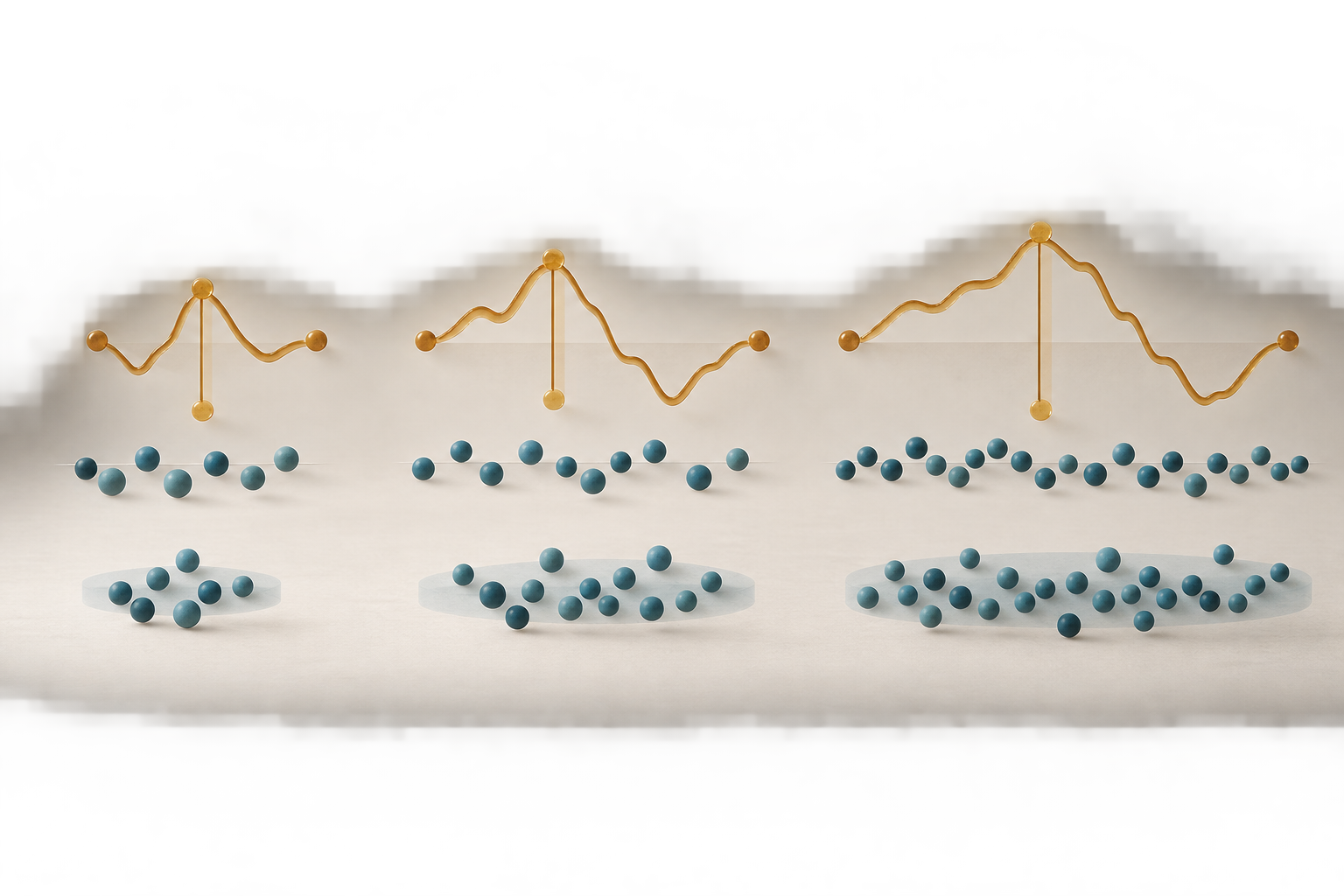
<!-- Illustration placement: after this section; text-free conceptual depiction of centered observations accumulating into a range at short and long block scales, with the range growing more than the within-block standard deviation. No axes, labels, or numeric claims. -->
Values around one half need a model and uncertainty interval
For a stationary series with finite variance and short-range dependence, many common long-run scaling results lead to an exponent near \(0.5\). Under a fractional Gaussian-noise-style model, \(H>0.5\) is consistent with positive long-range dependence: deviations tend to be followed by same-direction deviations more often than under the benchmark, with correlations decaying slowly. An exponent below \(0.5\) is associated with anti-persistence, where reversals or opposite-signed dependence dominate the scaling behavior.
The qualification “under the model” matters. The ordinary R/S slope is an estimate, not a direct test of one uniquely defined economic mechanism. Small-sample bias can move estimates away from \(0.5\); overlapping blocks, denominator conventions, scale endpoints, and autocorrelation affect the result. A confidence interval that includes \(0.5\) does not prove independence, and an interval that excludes it does not prove that a stable long-memory model generated the observations.
Do not translate \(H=0.7\) into “70% chance of trend continuation,” “returns persist for 70 days,” or “a 70% success rate.” \(H\) is not bounded to represent a probability or a holding period. It describes an estimated scaling relationship. Statistical evidence of dependence still needs a model, uncertainty assessment, and checks against alternatives such as short-run correlation, conditional heteroskedasticity, a deterministic trend, or a regime shift.
Short-run autocorrelation and clustered volatility can mimic persistence
Classical R/S responds to more than genuine long-range dependence. A short-lived AR pattern can keep same-signed deviations near one another and increase the cumulative range. Lo showed that short-range serial correlation can bias the classical statistic upward, making a short-memory process look persistent. His modified R/S method was designed to test for long memory while accounting for short-range dependence. In the stock-return indexes he examined, evidence of long memory disappeared after short-term autocorrelation was taken into account; that is a result for his samples and test, not a verdict on every asset or later period. See Lo’s 1991 paper.
Volatility clustering creates a different trap. A sequence can alternate positive and negative returns while the sizes of those returns remain clustered. R/S applied to returns asks about signed cumulative deviations; applied to absolute or squared returns it asks about persistence in magnitude. A high estimate for \(|r_t|\) can describe clustered risk without implying that price direction is predictable. For a separate diagnostic of conditional variance dependence, see the guide to the ARCH LM test. The variance-ratio guide addresses another summary of return dependence across horizons.
Heavy tails and outliers also matter. Mandelbrot and Wallis found useful robustness properties across many non-Gaussian simulations, but that does not mean a single extreme move, a volatility regime change, or an incorrectly specified mean is harmless. A sound analysis reports results on the chosen original series and examines how they change under justified alternatives, rather than removing inconvenient observations until the exponent looks familiar.
Trends, breaks, and the chosen scales can create false long memory
Subtracting the block mean removes a constant level from each block; it does not remove every deterministic or changing pattern. A gradual trend, a one-time level shift, a change in sample composition, or a volatility break can create a long cumulative excursion. The fitted log–log relationship may then look like a power law even though the series has no stable long-memory mechanism. A break test or segmented-regression analysis asks a different question; see the guide to interrupted time-series regression.
Scale choice is part of the model. Very short blocks mainly reflect local noise and microstructure; very long blocks leave few usable segments. Using overlapping windows can increase the number of computed ratios but does not create equally many independent pieces of information. An apparent crossover—one slope for short scales and another for longer scales—may signal different dynamics, a break, seasonal structure, or simply estimation noise. It should not be collapsed into one \(H\) without explanation.
Be explicit about whether the input is price, log price, return, absolute return, or a filtered residual, and whether blocks are overlapping or disjoint. Choose the block range and minimum block count before interpreting the outcome, report the observations contributing at each scale, and show sensitivity to reasonable endpoints. If prices are integrated, the usual interpretation for stationary returns does not carry over unchanged. Detrending is not a universal cure: it changes the object being measured and may remove economically meaningful variation along with nuisance trend.
Lo’s modified R/S changes the variance scale in the denominator
Lo’s modification keeps the range of centered cumulative deviations but replaces the ordinary block standard deviation with an estimate of long-run variance that includes short-lag autocovariances. A common notation is:
\[ Q_n^{\mathrm{Lo}}(q)=\frac{R_n}{\widehat{\sigma}_n(q)},\qquad \widehat{\sigma}_n^2(q)=\widehat{\gamma}_0+ 2\sum_{j=1}^{q}\left(1-\frac{j}{q+1}\right)\widehat{\gamma}_j. \]
Here \(\widehat{\gamma}_j\) is the sample autocovariance at lag \(j\), and \(q\) is the truncation bandwidth. The triangular weights give less weight to autocovariances nearer the cutoff. The modified statistic is compared with its appropriate null distribution; it is not simply the classical R/S estimate with a better-looking denominator, and its value is not automatically an adjusted \(H\).
The bandwidth controls which short-run correlations enter the variance estimate. Too small a \(q\) can leave relevant short-range dependence untreated; too large a \(q\) makes the estimate noisy and may absorb patterns that the analysis intended to distinguish. Report the bandwidth rule, sample frequency, test statistic, null, and p-value, and consider a prespecified sensitivity range. Lo’s paper shows why this distinction is material: classical R/S can react to short memory, while the modified test targets a broader null that permits weak short-run dependence.
DFA and frequency-domain estimates use different transformations
Detrended fluctuation analysis (DFA) first forms an integrated profile from mean-centered observations, partitions that profile into windows, fits a local polynomial within each window, and calculates the root-mean-square residual fluctuation \(F(s)\) at window size \(s\). A regression of \(\log F(s)\) on \(\log s\) estimates a scaling slope. The local fit can reduce sensitivity to selected polynomial trends, but the detrending order, window lengths, and series type still matter. DFA is not immune to breaks, volatility changes, or a scale interval chosen after inspecting the plot.
Frequency-domain methods estimate low-frequency behavior from the periodogram. Under a particular stationary long-memory model, if spectral power near frequency zero follows \(f(\lambda)\propto|\lambda|^{-\beta}\), then \(H=(\beta+1)/2\) for a fractional-noise-style return process. The low-frequency bandwidth determines which observations influence the fitted slope; seasonal peaks, breaks, and a small number of low-frequency ordinates can dominate it. The relation between a spectral parameter and \(H\) depends on whether the input is a stationary increment series or an integrated level.
These methods are alternative estimators with different finite-sample behavior, not three independent confirmations by default. Weron’s finite-sample comparison (DOI 10.1016/S0378-4371(02)00961-5) examined R/S, DFA, and periodogram regression using simulated Gaussian white noise and emphasized that estimates and confidence intervals differ by method and sample length. The results do not establish that DFA is always best on financial data; they show why inference should be calibrated for the actual procedure and data-generating conditions.
A trading hypothesis needs out-of-sample evidence after costs
An estimated exponent can help describe a historical scaling pattern or motivate a clearly stated hypothesis. It does not supply entry and exit rules, forecast timing, position size, risk limits, or a reason why any measured relationship should persist after it becomes known. If a researcher tests whether a trailing \(H\) estimate predicts returns, the prediction horizon and decision time must be fixed before evaluation, and every input must have been available at that time.
Rolling many window lengths, block sizes, assets, return transforms, detrending orders, and thresholds until one shows a high \(H\) is multiple testing. The apparent winner has been selected from the same data used to evaluate it. Treat the entire search as part of the research record; use untouched or properly forward-chained evaluation and account for the candidate search. The guides to probability of backtest overfitting and White’s Reality Check discuss related selection problems.
A statistical association is not a net trading edge. A strategy must be evaluated after bid–ask spread, commissions, slippage, market impact, funding or financing, borrow costs, and turnover. Persistent volatility can raise risk and drawdowns without improving the direction of returns. Report the estimate’s uncertainty, compare it with short-memory and break alternatives, freeze the rule before the final test, and distinguish a historical diagnostic from a strategy result.
Resampling only helps when its design matches the dependence being studied. An iid bootstrap that draws individual returns independently destroys their time order. A block bootstrap retains local runs within each chosen block, but a short block may miss slow dependence and a long block leaves fewer effectively distinct pieces; neither makes a structural break disappear. If a scale, window, or asset was selected from the data, repeat that selection inside every resample when estimating search-adjusted uncertainty. Resampling only the final selected exponent understates the uncertainty created by the search.
Common questions
Q1What does a Hurst exponent above 0.5 mean?
Under common stationary-increment scaling models, it is consistent with persistent dependence in the measured series over the scales analyzed. It does not mean a 50% or 70% chance of a price rise, nor does it prove a profitable signal.
Q2Is R/S analysis the same as Lo’s modified R/S test?
No. Classical R/S divides the cumulative-deviation range by ordinary within-block variation. Lo’s modified statistic uses a long-run variance estimate that includes weighted short-lag autocovariances and is tested against a null that allows short-run dependence.
Q3Can the Hurst exponent be used to choose a trading strategy?
It can motivate a research hypothesis, but the estimate alone gives no entry, exit, or sizing rule. Any proposed strategy needs a frozen specification, uncertainty and alternative-model checks, out-of-sample evaluation, and realistic execution costs.
Sources and further reading
Report an issue
We’ll prepare an email with this article link. Mark receives the report only after you send it
Quick check
Read the guide? Check yourself with 3 questions
Question 01
What does the slope in a log R/S-versus-log block-length fit estimate?
Choose an answer to see the explanation