Roll Bid–Ask Spread Estimator: Formula, Example, and Limits

A quoted spread is the ask minus the bid at a particular time. An effective spread instead summarizes the cost faced by trades that actually occurred relative to a contemporaneous midpoint. The Roll estimator is a low-frequency proxy for that effective spread: it uses the serial covariance of observed transaction-price changes to infer the price gap that may have caused short-run reversals.

The attraction is a limited data requirement. If reliable transaction prices are available but historical bid and ask quotes or trade-direction flags are not, the estimator can still be calculated. That makes it useful for historical comparisons and for markets where quote archives are incomplete. It does not reconstruct the quote book, identify each trade’s side, or tell a trader the spread available now. Roll’s original paper derives the measure for an efficient market and notes that the estimated object is an effective spread rather than necessarily the displayed quoted spread (Roll, 1984).

The estimate is also not a complete transaction-cost measure. It does not include commissions, market impact from a particular order, the cost of waiting, unfilled quantity, or a price move after the observation. Treat it as one model-based summary of historical transaction-price behavior, not as an executable quote or a full backtest cost model.

Let \(x_t\) be the log transaction price, \(m_t\) the unobserved log value around which the bid and ask are centered, and \(s\) the full effective spread in log-price units. In the simple symmetric model,

\[ x_t=m_t+\frac{s}{2}q_t, \]

where \(q_t=+1\) for a buyer-initiated trade at the ask and \(q_t=-1\) for a seller-initiated trade at the bid. The observed return is therefore

\[ r_t=\Delta x_t=\Delta m_t+\frac{s}{2}(q_t-q_{t-1}). \]

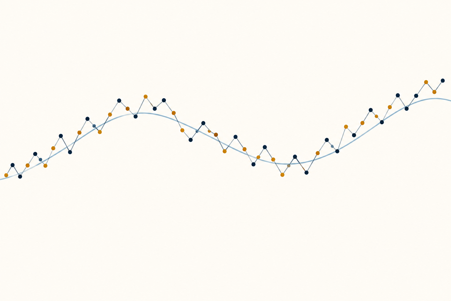
Suppose trade signs are independent and equally likely to be \(+1\) or \(-1\), efficient-value innovations have no serial covariance, and the spread is constant over the sample. When a transaction switches from one side to the other, the transaction price moves across the spread even if the underlying value barely changes. A buy at the ask followed by a sell at the bid creates a negative return followed by a positive reversal, or the reverse sequence. If the same side trades twice, the spread component may be zero across those observations.

Under these assumptions, the spread component makes consecutive returns move in opposite directions on average:

\[ \operatorname{Cov}(r_t,r_{t-1})=-\frac{s^2}{4}. \]

Solving for \(s\) gives the Roll formula. The covariance pattern is an implication of the model, not proof that every observed price reversal comes from the bid–ask spread.

<!-- Illustration placement: after section 3; text-free conceptual comparison of a smooth underlying value path with transaction prices alternating above and below it. No labels, axes, or values. -->

Write the first-order covariance as \(C_1=\operatorname{Cov}(r_t,r_{t-1})\). Given a sample of \(T\) returns, one common sample convention is

\[ \widehat C_1=\frac{1}{T-1}\sum_{t=2}^{T}(r_t-\bar r)(r_{t-1}-\bar r), \]

where \(\bar r\) is the sample mean. If \(\widehat C_1<0\), the plug-in estimate is

\[ \widehat s_{\text{Roll}}=2\sqrt{-\widehat C_1}. \]

The result has the same units as the returns used in the covariance. If \(r_t\) is a log return, \(\widehat s\) is a proportional or log-price spread. If the input is a dollar price change rather than a return, the estimate is in price units. State the transformation, sampling interval, and covariance convention before comparing estimates across assets or periods.

Roll emphasizes covariance rather than correlation. Correlation divides by the unconditional return variance, which includes variation from new information in the efficient value. That news-driven variance can change even when the spread mechanism does not. The unnormalized covariance has the model’s direct relationship to the squared spread; replacing it with an autocorrelation changes the estimator and its interpretation. If a study uses log prices, scaled returns, or a different denominator, show that convention explicitly.

Suppose a hypothetical sample of transaction-price log returns is expressed in basis points and its demeaned first-order sample covariance is \(-1.44\,\text{bp}^2\). The estimate is

\[ \widehat s_{\text{Roll}}=2\sqrt{-(-1.44)}=2\sqrt{1.44}=2(1.20)=2.40\,\text{bp}. \]

This is a full proportional-spread estimate of \(2.40\) basis points, or \(0.024\%\), under the model. At a hypothetical midpoint of \(\$100\), the small-spread dollar conversion is approximately

\[ \$100\times 0.00024=\$0.024 \]

per share for the full spread. Half of that is about \(\$0.012\) per share from midpoint to one side. If quotes stayed unchanged and a trader bought at the ask then sold at the bid for 1,000 shares, the full-spread price difference would be about \(\$24\), before commissions, other fees, price movement, or market impact. Those are illustrative conversions, not observed quotes or a promised execution cost.

The arithmetic does not show whether \(\$100\) was an executable midpoint, how much quantity was available, or what an order would have paid. A Roll estimate can smooth a historical sample into one statistic while hiding variation by time of day, order size, or market state. Do not compare the estimate with a current displayed spread unless the asset, interval, and spread definition match.

A constant \(s\) is a simplifying assumption. Roll also considers a spread that changes over time and derives a relation to the average squared spread under the model. In that setting, applying the square-root formula corresponds to a root-mean-square spread, not generally the arithmetic average spread. A few wide-spread observations can therefore influence the estimate disproportionately because the spread enters through its square.

The original model also gives a result that can sound broader than it is: under its assumptions, the expected spread-induced covariance is invariant to the length of a nonoverlapping observation interval. That is not a promise that daily, weekly, and intraday empirical estimates will match. Real trade signs can persist across observations, some intervals contain no trades, and spread conditions vary. Changing the interval also changes which transaction becomes the sampled price and how much information noise enters each return.

Choose the sampling rule before looking at the result. For example, compare consistently sampled transaction prices rather than mixing official closing trades, midpoint marks, and stale last prices. Identify whether returns span calendar time or trading sessions, how holidays and nontrading periods are handled, and whether corporate actions or contract rolls were adjusted. A different sample interval is a different empirical design even when the same formula is applied.

The square root is real only when the sample covariance is negative. If \(\widehat C_1=0\), the plug-in calculation returns zero; if \(\widehat C_1>0\), the basic formula is undefined. A zero or positive sample covariance is not evidence that the true spread is zero. It may reflect sampling noise, persistent trade direction, price discreteness, serial dependence in efficient-value returns, or a spread too small to distinguish from the noise in a short sample.

Some empirical implementations replace a positive covariance with zero before taking the square root. Others use an absolute value or report only windows with negative covariance. These choices can produce a number, but they are extra rules, not consequences of the Roll equation. Report how many estimates were undefined, how often the estimate was set to zero, and whether exclusions changed the sample. Silently taking an absolute value can turn a covariance that contradicts the model into a positive spread estimate.

Small samples add another problem. The covariance itself is estimated with error and then transformed by a square root. Harris derives finite-sample properties under the Roll model and shows that noise can make sample covariances positive and that the nonlinear transformation can cause material bias (Harris, 1990). A point estimate should be accompanied by its sample length and sensitivity to reasonable windows; it should not be presented with more precision than the price data support.

The simple derivation requires more than a negative covariance. It assumes independent, equally likely buy- and sell-initiated trades; a symmetric spread around an efficient value; no serial covariance in efficient-value innovations; and a sampling process that represents the transaction-price mechanism. Market order splitting and inventory management can make trade signs persistent. If buyers tend to arrive in runs, transaction returns can retain a positive spread-related component and the negative covariance can be weaker than the model predicts.

The midpoint path can also have serial dependence. Momentum, reversal, stale prices, asynchronous observations, or scheduled price adjustments may create negative or positive return covariance even without a corresponding change in the effective spread. Price discreteness and tick-size effects can create reversals of their own. These effects do not have to dominate the sample to matter: the estimator infers spread from one moment, so any other process affecting that moment can confound the result.

Time variation creates a further distinction between a sample average and a stable market property. The spread can widen around news, open and close, thin trading, or market stress. A full-period estimate can hide those episodes; short windows can instead be too noisy to estimate covariance. Examine the time series and report the window definition. The negative serial covariance is consistent with bid–ask bounce under the model; it is not a causal decomposition of all short-run price movement.

If reliable quote and trade data are available, a direct effective-spread calculation can compare each trade price with a contemporaneous midpoint and account for trade direction. That requires synchronized, cleaned observations and a clear rule for locked, crossed, stale, or out-of-sequence quotes. It measures the observed trades in that data set, whereas Roll infers a spread from the serial covariance of transaction prices. A trade-direction classification guide explains why trade signs themselves may need an estimation rule.

Other low-frequency methods use different information and assumptions. Hasbrouck develops a Gibbs-sampler estimate from daily closing prices rather than relying only on the basic Roll plug-in transformation (Hasbrouck, 2009). Corwin and Schultz use daily high and low prices to construct a spread estimator without relying on the same trade-direction dynamics (Corwin and Schultz, 2012). These alternatives do not make the quoted spread observable from any price series; their estimates have their own assumptions and validation scope.

The practical question determines the measure. For historical cross-market comparisons with limited quote data, a low-frequency proxy may be useful if its failure rate and assumptions are reported. For an order decision, inspect current bid, ask, depth, and order size. The futures spread and slippage guide distinguishes a quoted spread from realized execution differences, while the ETF liquidity guide discusses why volume alone does not describe executable liquidity.

A reproducible report should state whether the observations are trades, official closes, or another transaction-price proxy; whether the input uses price changes or log returns; the sampling interval; the number of observations; the covariance denominator; and the treatment of zero or positive covariance. Also specify the asset universe, date range, corporate-action and roll adjustments, data filters, and whether the spread is reported in price, percentage, or basis-point units. If spread stability is implausible, show estimates across prespecified subperiods rather than selecting the window with the most negative covariance.

A Roll estimate is a historical transaction-cost proxy under a model. It does not reveal today’s quote, guarantee an execution price, measure the full cost of a strategy, or forecast the next return. A trader evaluating a backtest still needs an order-size-aware model for spread, commissions, market impact, partial fills, and timing. A lower estimated spread is not itself evidence of a tradable edge. For a broader view of observed volatility at different sampling frequencies, see the guide to realized volatility.