

Hayashi–Yoshida Covariance Estimator: Asynchronous Prices Explained
Learn how the Hayashi–Yoshida estimator uses overlapping return intervals to estimate integrated covariance when assets trade at different times, and where the method stops
In this guideWhy asset-price covariance becomes difficult when trading clocks differ
Short summary
The Hayashi–Yoshida (HY) estimator measures integrated covariance from two price series whose observations arrive at different times. It pairs return increments when their time intervals overlap, so it does not first have to interpolate one asset’s price onto the other asset’s timestamps. In its classical form, HY addresses nonsynchronous sampling under a diffusion model; it does not remove market microstructure noise or turn a covariance estimate into a forecast.
Why asset-price covariance becomes difficult when trading clocks differ
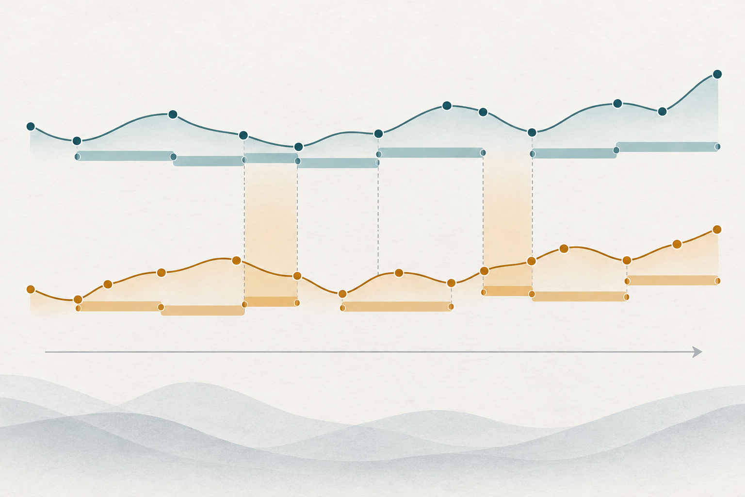
Two assets can share market hours and still trade at different instants. A liquid stock may print many times while a less active stock has no new trade or quote. Their observed price changes then form separate time grids. The statistical target may be the assets’ contemporaneous covariation, but no single pair of observed returns necessarily covers the same interval.
A familiar alternative is to put both series on a regular clock by carrying the last observed price forward. This creates aligned return columns, but an unchanged carried-forward price is not a new independent observation of the latent price. The resulting zero returns and delayed catch-up moves can distort measured co-movement. Epps documented that observed stock-return correlations can decrease as the measurement interval gets shorter; nonsynchronous observations are one important mechanism, alongside other market-data effects. That short-interval pattern is commonly called the Epps effect (Epps, 1979).
Hayashi and Yoshida proposed an estimator that works with the original nonsynchronous increments instead of choosing an interpolation rule first. Their original study established consistency for diffusion prices under high-frequency sampling conditions (Hayashi & Yoshida, 2005); a later paper derived asymptotic normality under a general nonsynchronous sampling scheme (Hayashi & Yoshida, 2008). The central idea is simple to state but easy to misuse: match increments by overlapping time intervals, not merely by nearby timestamps.
Define the covariance target before calculating it
Let \(X_t\) and \(Y_t\) be the latent efficient log prices of two assets over a common horizon \([0,T]\). In a simple continuous diffusion model, write
\[ dX_t=\mu^X_t\,dt+\sigma^X_t\,dW^X_t,\qquad dY_t=\mu^Y_t\,dt+\sigma^Y_t\,dW^Y_t, \]
with instantaneous Brownian correlation \(d[W^X,W^Y]_t=\rho_t\,dt\). The target is the integrated covariation
\[ [X,Y]_T=\int_0^T \sigma^X_t\sigma^Y_t\rho_t\,dt. \]
This is a path quantity accumulated over the chosen observation window. It is not the covariance of two static price levels, and it is not automatically a correlation. Its units are the product of the two return units: if both log returns are expressed in percentage points, the estimate is in percentage-point squared. The realized-volatility calculation guide covers the univariate squared-return measure, while the quadratic-variation guide explains the path quantity that multivariate realized covariance extends.
The target can be positive or negative. Positive integrated covariation means that same-window price increments tended to contribute cross-products with the same sign; negative covariation means opposite-signed cross-products dominated. Neither sign by itself establishes why the assets moved together, whether one caused the other, or whether a portfolio rule would be profitable.
Why previous-tick synchronization can distort the estimate
To calculate ordinary realized covariance, an analyst may choose regular clock times and use the latest available price for each asset. That is convenient, but the answer can depend on the grid width and interpolation convention. When a price is stale, several grid observations repeat the same quote. A later update may then appear as one return spanning more time than its paired return in the other asset.
This can move contemporaneous covariance into apparent lead–lag terms or attenuate it toward zero as the grid becomes finer. Epps’s original empirical result describes the short-interval change in observed co-movement; later work derives bias in previous-tick covariance when sampling is nonsynchronous and observed prices also contain noise. So an observed high-frequency correlation decline is a diagnostic pattern, not proof that asynchronous timing is the only cause.
HY avoids a particular synchronization choice by retaining each observed return’s own interval. It does not make timestamp quality irrelevant: both assets still need a common clock, correct session boundaries, and a clear rule for the start and end of the horizon. It also does not fix noisy transaction prices, bad quotes, or a target that mixes different trading sessions.
Pair returns when their observation intervals overlap
Suppose asset \(X\) is observed at \(0=t_0<t_1<\cdots<t_n=T\), and asset \(Y\) at \(0=s_0<s_1<\cdots<s_m=T\). Their observed log-return increments are
\[ \Delta X_i=X_{t_i}-X_{t_{i-1}},\qquad \Delta Y_j=Y_{s_j}-Y_{s_{j-1}}. \]
Associate each return with its time interval, \(I_i=(t_{i-1},t_i]\) and \(J_j=(s_{j-1},s_j]\). The HY estimator is
\[ \widehat{[X,Y]}^{HY}_T =\sum_{i=1}^{n}\sum_{j=1}^{m} \Delta X_i\,\Delta Y_j\, \mathbf{1}\{|I_i\cap J_j|>0\}. \]
The indicator includes a cross-product when the two return intervals overlap for a positive amount of time. An exact shared endpoint alone does not count as an overlap of positive duration. Each increment can overlap more than one increment from the other asset, and each such cross-product is included once. The procedure neither fills forward prices nor splits a return into invented sub-returns.
Under the classical continuous-diffusion setup, with sufficiently fine observation intervals and suitable sampling conditions, the sum converges to integrated covariation as the maximum interval length shrinks. The original result is about nonsynchronous observation; it assumes the observed prices are not corrupted by the market microstructure noise that often appears in raw tick data.
<!-- learn:illustration -->
Reproduce a small hypothetical overlap calculation
Suppose two assets are observed over the same five-unit session. The table lists hypothetical log returns in percentage points and the interval each return covers. The observation times are staggered, so the return endpoints do not all match.
| Asset X interval | Return | Asset Y interval | Return | Overlap product |
|---|---|---|---|---|
| \((0,1.8]\) | \(+0.40\%\) | \((0,1.0]\) | \(+0.30\%\) | \(+0.12\ \mathrm{pp}^2\) |
| \((0,1.8]\) | \(+0.40\%\) | \((1.0,2.4]\) | \(+0.50\%\) | \(+0.20\ \mathrm{pp}^2\) |
| \((1.8,3.2]\) | \(+0.20\%\) | \((1.0,2.4]\) | \(+0.50\%\) | \(+0.10\ \mathrm{pp}^2\) |
| \((1.8,3.2]\) | \(+0.20\%\) | \((2.4,3.9]\) | \(-0.20\%\) | \(-0.04\ \mathrm{pp}^2\) |
| \((3.2,5]\) | \(-0.10\%\) | \((2.4,3.9]\) | \(-0.20\%\) | \(+0.02\ \mathrm{pp}^2\) |
| \((3.2,5]\) | \(-0.10\%\) | \((3.9,5]\) | \(+0.10\%\) | \(-0.01\ \mathrm{pp}^2\) |
For example, the first \(X\) interval overlaps the first \(Y\) interval from 0 to 1.0 and the second from 1.0 to 1.8, so both cross-products enter. The next \(X\) return overlaps the second \(Y\) return from 1.8 to 2.4 and the third from 2.4 to 3.2. The final pair of \(X\)-overlaps contributes \(0.02-0.01\ \mathrm{pp}^2\). Summing the six included products gives
\[ \widehat{[X,Y]}^{HY}_T =0.12+0.20+0.10-0.04+0.02-0.01 =0.39\ \mathrm{pp}^2. \]
Because one percentage point is \(0.01\) in decimal-return units, \(0.39\ \mathrm{pp}^2=3.9\times10^{-5}\) in decimal log-return-squared units. These inputs are invented solely to make the arithmetic reproducible. The result is a cumulative covariance estimate for this window, not a percent return, a correlation, or a market observation.
Interpret the sign and scale without turning covariance into a signal
The example’s positive sum says that, across the overlapping intervals, positive-positive and negative-negative products outweighed the negative products. It does not mean either asset rose by 0.39%, and it does not say that 39% of their moves were shared. Covariance scales with the return units and with the length and activity of the window; a larger number can reflect a different unit or horizon rather than stronger standardized dependence.
Correlation is dimensionless and requires covariance to be scaled by volatility estimates. A simple ratio built from separately sampled or separately estimated variance terms is not automatically a valid correlation estimate. In finite samples, the resulting ratio can even fall outside \([-1,1]\). The integrated covariance alone also cannot distinguish common news, delayed price adjustment, common exposure, or other mechanisms.
For a portfolio application, state the asset weights, horizon, return units, and covariance convention. Do not treat a positive HY estimate as a long signal or a negative estimate as a hedge instruction. The forex-pair correlation guide explains why correlation and shared exposure still need careful interpretation. A historical realized measure describes the selected data window; it does not predict the next return or guarantee that a hedge will offset future losses.
Know the sampling and price assumptions behind classical HY
The classic estimator was developed for diffusion-type prices observed at discrete, nonsynchronous times. A practical approximation needs enough observations that the largest gap in each series is small relative to the analysis window. Long no-trade gaps leave wide returns whose cross-products cover many possible movements; the formula can still be computed, but the fine-sampling approximation may be weak.
Observed transaction prices often contain bid–ask bounce, price discreteness, stale quotes, latency, and other measurement effects. HY’s overlap rule solves the timing mismatch; it does not remove these price errors. Griffin and Oomen study realized covariance, lead–lag adjustments, and HY under asynchronous sampling with iid microstructure noise, and show that relative finite-sample performance depends on noise and correlation conditions (Griffin & Oomen, 2011). Their analysis is a warning against describing plain HY as generally noise-robust.
The model also requires a defensible common horizon. If one market closes before the other, using a nominally identical calendar window may pair returns that do not represent the same active trading period. Time-zone conversion, daylight-saving transitions, auction prints, corporate actions, missing intervals, and outlier filtering can all alter the overlap set. Document these choices instead of treating timestamps as bookkeeping details.
Choose inference and noise treatment separately from the point estimator
A point estimate is not a confidence interval. Hayashi and Yoshida later established asymptotic normality under a general nonsynchronous sampling scheme, but an applied standard error still needs a feasible variance estimator and assumptions that match the sampling design. Sparse or highly uneven observations can make uncertainty large even when the overlap sum looks stable.
For noisy high-frequency prices, use a method designed for both noise and nonsynchronicity, or justify a sampling and preprocessing rule that limits noise. Christensen, Kinnebrock, and Podolskij develop pre-averaging covariance estimators for noisy diffusion models with nonsynchronous data, including a pre-averaged HY-type estimator that can be applied without first aligning the raw prices (Christensen et al., 2010). Barndorff-Nielsen and coauthors’ multivariate realized kernels target covariation under noise and nonsynchronous trading and are constructed to yield positive-semidefinite covariance estimates (Barndorff-Nielsen et al., 2011). The realized-kernel estimator guide explains that alternative in more detail.
That matrix property matters when a portfolio optimizer or risk system requires a coherent covariance matrix. Pairwise HY estimates calculated on different overlap sets do not by themselves guarantee that the assembled matrix is positive semidefinite. Do not silently “repair” the matrix by changing eigenvalues: report any projection, shrinkage, or alternative estimator as a separate modeling step. Noise-robust estimators also have tuning choices and assumptions; they are not automatic corrections for every market-data defect.
Report a reproducible estimate and its limits
A useful report names the two price series, whether they are trades, quotes, or midpoints, the common clock and session, the start and end of \([0,T]\), the return transformation, the overlap convention, the sampling-gap summary, and the estimator used. Show the covariance units and window. State how stale observations, outliers, jumps, auctions, and market microstructure noise were handled. If the inputs are asynchronous, disclose whether the analysis used raw intervals or first synchronized prices.
Do not annualize an integrated covariance by habit. If converting a window estimate into a rate or an annualized number, state the time-scaling assumption and how overnight periods and market closures are treated. If it is used to estimate correlation, state the variance estimators in the denominator and check the resulting matrix constraints. These reporting choices affect interpretation as much as the overlap formula does.
The Hayashi–Yoshida estimator is useful because it gives a direct, reproducible way to accumulate cross-products from nonsynchronous intervals without inventing synchronized prices. Its classical guarantee is conditional on a suitable noise-free diffusion framework and dense-enough sampling. It does not establish causality, solve market microstructure noise, or promise a reliable hedge or trading rule. Keep those boundaries with the estimate.
Common questions
Q1Does the HY estimator require both assets to trade at the same instant?
No. That is the timing mismatch it is designed to handle. It multiplies returns when their time intervals overlap, even if their observation timestamps differ.
Q2Does HY work directly on noisy transaction prices?
The classical estimator addresses nonsynchronous sampling under a diffusion model, not arbitrary market microstructure noise. Bid–ask bounce, discrete prices, stale quotes, and related effects may require a separate noise-robust method or a carefully justified sampling procedure.
Q3Is the HY estimate a correlation?
No. It estimates integrated covariance, which has units equal to the product of the return units. A correlation requires volatility scaling, and finite-sample estimates built from asynchronous inputs may not obey all correlation-matrix constraints.
Q4Can I use a positive HY estimate as a trading signal?
Not by itself. It summarizes cross-products over a historical window; it does not show causality, forecast future co-movement, or account for execution costs and changing risk.
Sources and further reading
Report an issue
We’ll prepare an email with this article link. Mark receives the report only after you send it
Quick check
Read the guide? Check yourself with 3 questions
Question 01
Which return pairs enter the classical Hayashi–Yoshida sum?
Choose an answer to see the explanation
Options glossary
Volatility calculated from price changes that occurred under a stated return, sampling-window, and annualization rule; different conventions can produce different values.
Read the deeper guideQuadratic variationThe limit of sums of squared process increments over increasingly fine partitions, measuring accumulated second-order path variation and generating Itô corrections.
Read the deeper guide