

Parkinson, Garman–Klass, Rogers–Satchell, and Yang–Zhang: OHLC Volatility Estimators
Compare four OHLC volatility formulas, see how each treats price ranges and opening gaps, and work through a hypothetical three-session example
In this guideWhat information an OHLC bar adds
Short summary
Parkinson, Garman–Klass, Rogers–Satchell, and Yang–Zhang use the high, low, open, and close to estimate historical variance from more than closing prices alone. Their formulas answer different measurement questions: the first two assume a continuous, no-drift session, Rogers–Satchell allows drift within that session, and Yang–Zhang adds the move from the prior close to the next open
What information an OHLC bar adds
An OHLC bar records the opening price O, highest observed price H, lowest observed price L, and closing price C over a defined interval. A close-to-close return keeps only the change between two endpoints. The high and low also say how far price travelled inside the interval, even when it ended near where it began
That extra path information can make a range estimator more statistically efficient when the price process resembles the model used to derive it. It does not make every OHLC estimate better in every market. A printed high or low can be a bad tick, a thin-market trade, a limit-up or limit-down print, or an auction price. Jumps and changing volatility also violate assumptions behind the classic formulas
The word “volatility” is often used for either variance or its square root. The formulas below first produce a variance estimate in squared log-return units for one bar. Take its square root to get that bar's volatility. Keep the distinction explicit: averaging standard deviations is not the same operation as averaging variances and then taking a square root
Define the price interval before calculating
Use a consistent O, H, L, C for every interval, with H at least as high as O and C and L at most as low as both. Apply the same price adjustment and currency convention to all four values. A stock split, distribution adjustment, contract roll, token redenomination, or a mismatch between venues can create an artificial range if only some prices are adjusted
For a bar i, define hᵢ = ln(Hᵢ/Lᵢ), cᵢ = ln(Cᵢ/Oᵢ), uᵢ = ln(Oᵢ/Cᵢ₋₁), and dᵢ = ln(Cᵢ/Oᵢ). The open-to-close term cᵢ and dᵢ are the same return; uᵢ is the between-bar return from the previous close to this open. Natural logarithms make the terms additive across adjacent price intervals
An exchange session can close while the underlying news and other venues keep moving. The next open may therefore sit above or below the previous close. A formula built only from H/L inside each session does not see that gap. Continuous crypto markets have no overnight closure, but the boundary between two daily bars still depends on the chosen timezone and cutoff; do not label every boundary move an overnight gap
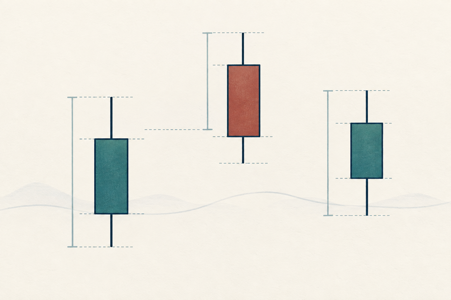
Parkinson: use the high-low range alone
Parkinson's estimator for n equal intervals is σ²P = (1/n) Σᵢ[ln(Hᵢ/Lᵢ)]² ÷ (4 ln 2). It asks how wide the observed range is, not where the interval opened or closed. The original paper derives the range method for a continuous random walk with zero drift ([Parkinson's paper]({source:parkinson1980ExtremeValueVariance})); its appeal is that a high-low range can contain more information about diffusion variance than a single close-to-close change
For a single interval with H/L = 104/98, ln(104/98) is about 0.05942. Squaring it and dividing by 4 ln 2 gives an estimated interval variance of about 0.001274; the square root is about 3.57% for that interval. This is a model-based estimate, not a claim that the price actually followed a smooth path or that the next interval will move 3.57%
Because Parkinson does not use O or C, it cannot distinguish a session that opened near its low and closed near its high from one that reversed. It also omits the prior-close-to-open move. If drift during the interval is material, the zero-drift derivation can bias the estimate. The range becomes especially fragile when highs and lows are affected by jumps, sparse trading, stale quotes, or bad prints
Garman–Klass: add the open-close movement
The classic Garman–Klass per-interval component is gᵢ = 0.5[ln(Hᵢ/Lᵢ)]² − (2 ln 2 − 1)[ln(Cᵢ/Oᵢ)]². Average gᵢ across n intervals to estimate variance. It uses the range and the open-to-close movement together; when the close-to-open move is large relative to the high-low range, the second term adjusts what the range alone would imply
Using the example bar O=100, H=104, L=98, C=103, the first term is 0.5 × 0.05942² and the second is (2 ln 2−1) × ln(1.03)². The result is approximately 0.001428, or a 3.78% interval standard deviation after taking the square root. Keep all inputs as prices from one bar and use natural logs; mixing simple percentage changes with these log-return terms changes the estimator
Garman and Klass formulate improved estimates within a specified continuous price-process model ([their paper]({source:garmanKlass1980OhlcVolatility})). Its efficiency advantage is conditional on that model, not a universal ranking. A discontinuous opening gap is outside the intraday O-to-C path, and a jump inside the session can distort both the range and the open-close correction. When the data do not resemble the assumed path, the lower sampling variance claimed under the model does not guarantee lower real-world error
Rogers–Satchell: allow drift inside a bar
The Rogers–Satchell component is rsᵢ = ln(Hᵢ/Oᵢ)ln(Hᵢ/Cᵢ) + ln(Lᵢ/Oᵢ)ln(Lᵢ/Cᵢ). Average the components across intervals. Unlike the zero-drift range derivations, this estimator is unbiased for variance under the paper's continuous diffusion model with an arbitrary drift term ([Rogers and Satchell's paper]({source:rogersSatchell1991VarianceEstimator})). That makes the within-interval direction less of a problem when the price process is steadily trending
For the example O=100, H=104, L=98, C=103, the upper contribution is ln(1.04) × ln(104/103), and the lower contribution is ln(0.98) × ln(98/103). Their sum is approximately 0.001384, with a square root of 3.72%. The two products combine the high and low's location relative to both endpoints; this is why Rogers–Satchell is not just another way to square the range
Drift handling does not mean jump-proof, noise-proof, or gap-proof. Rogers–Satchell describes movement between O and C within the bar. If O is the next session's first trade, the previous close-to-open move is not part of that bar's component. Use a separate gap term or a method designed to include it when that exposure belongs in the measurement question
Yang–Zhang: separate the gap and session components
Yang–Zhang combines three pieces ([their paper]({source:yangZhang2000DriftIndependentOhlcVolatility})): sample variance of between-bar log returns uᵢ = ln(Oᵢ/Cᵢ₋₁), sample variance of open-to-close log returns dᵢ = ln(Cᵢ/Oᵢ), and the mean Rogers–Satchell component. One common notation is σ²YZ = s²u + k s²d + (1−k) mean(rsᵢ), where k = 0.34 ÷ [1.34 + (n+1)/(n−1)]. The sample variances use the sample mean and n−1 divisor; the Rogers–Satchell components are averaged over n intervals
This construction is meant to combine drift handling within the session with the movement between the previous close and next open. It is useful when that boundary move is economically part of the daily risk being measured. The formula requires at least two intervals for the sample-variance terms. The between-bar component captures the previous-close-to-open return; intrabar jumps, price discreteness, microstructure noise, and changing variance still affect the estimate
For a 24/7 market, “overnight” is shorthand at best. Define bars with a consistent cutoff, calculate the previous-close-to-next-open return at that boundary, and explain that the term is a between-bar return while trading continued. Comparing a UTC-day estimate with an exchange-session estimate can produce different numbers even on identical trades
Compare the estimates without treating them as signals
| Estimator | Inputs within each bar | Drift and gap treatment | A sensible use |
|---|---|---|---|
| Parkinson | H, L | Derived for zero drift; does not use O, C, or the prior-close gap | A compact range-only benchmark when its assumptions are plausible |
| Garman–Klass | O, H, L, C | Classic derivation assumes a continuous session without drift or jumps; excludes the prior-close gap | A range estimate that also accounts for the open-close move |
| Rogers–Satchell | O, H, L, C | Allows within-bar drift under continuous diffusion; excludes the prior-close gap | A session estimate when trend within the bar should not be treated as zero drift |
| Yang–Zhang | Prior C plus O, H, L, C | Separates between-bar and within-session returns; handles drift under its model | A daily estimate when the close-to-open move belongs in the risk measure |
Choose based on the object you want to measure, not on which result looks largest or smallest. Compare the OHLC estimates with close-to-close variance on the same price series, dates, interval, and annualization convention. If the methods diverge, inspect the actual ranges, open-close movement, gaps, outliers, and session definition instead of selecting the value that supports a preferred conclusion
Average true range (ATR) is related because it uses high, low, and the previous close, but it is not another estimator in this table. ATR averages a price-unit true range; these formulas estimate variance from log-price ratios. ATR can help express a stop distance under a chosen trading rule, while an OHLC variance estimate describes historical dispersion. Do not compare an ATR of $2 directly with a 3% standard deviation.
A hypothetical three-session calculation
Assume a prior close of 100 and three hypothetical sessions. Session 1 has O=100, H=104, L=98, C=103; session 2 has O=105, H=108, L=102, C=103; session 3 has O=101, H=106, L=99, C=105. These invented prices are only a reproducible arithmetic example, not live market data
Applying Parkinson to each H/L pair and averaging gives σ²P ≈ 0.0013785, or √σ²P ≈ 3.71% per session. Averaging the Garman–Klass components gives ≈ 0.0015566, or 3.95%. Averaging the Rogers–Satchell components gives ≈ 0.0015458, or 3.93%. These are daily-scale standard deviations from three bars; rounding explains small differences in the displayed figures
For Yang–Zhang, the three between-bar returns are 0.00000, ln(105/103)=0.01923, and ln(101/103)=−0.01961. Their sample variance is about 0.0003771. The open-to-close returns are ln(103/100)=0.02956, ln(103/105)=−0.01923, and ln(105/101)=0.03884; their sample variance is about 0.0009731. With n=3, k≈0.1018 and mean(rsᵢ)≈0.0015458. Substitution gives σ²YZ≈0.0018646 and √σ²YZ≈4.32% per session
The four results differ because their formulas assign different roles to the high-low range, open-close movement, and between-bar movement. Three observations are far too few for a stable estimate, and the example does not show that one estimator is more accurate. Recompute with a longer, consistently sampled series and report the period count, data source, outlier policy, and session cutoff
Diagnose the bars before trusting a rolling series
Review the bars that contribute most to the estimate instead of reading only the final number. A single extreme H or L enters squared log-range terms and can dominate a short window. Compare the raw trade or quote record, confirm that the high and low belong to the stated interval, and check whether a split, contract roll, venue outage, thin order book, or price-limit event changed the observed path. Removing an observation because it makes the result inconvenient is not a defensible outlier policy; record the rule before calculating
The opening price may also have a different data meaning across vendors. Some bars use the first eligible trade, some use an auction print, and some aggregate quotes or trades differently. If one feed starts the session at an auction and another starts at the first continuous-market trade, O and the apparent gap can differ even when later prices match. For daily or weekly history, verify whether the bar is adjusted and whether its timestamp denotes the start or end of the interval
For a rolling estimate, record both the lookback length and update frequency. A 20-session estimator updated every session shares 19 of 20 observations with its prior value, so adjacent estimates are not independent. A smoothing rule may make the displayed curve easier to read, but it adds another model choice and delay. Keep the raw estimator available so a smoothed chart cannot hide a jump, data outage, or abrupt change in the underlying range
Convert units and use the estimate carefully
The worked values are per-session variance and standard deviation. To express a variance estimate as an annualized volatility, first multiply variance by the number of comparable sessions per year and then take the square root. A U.S. equity workflow may use 252 trading sessions; a continuously traded crypto series may use 365 daily bars if that definition suits the research question. Neither count is universal, and annualization does not repair a mismatched bar definition or a jump-contaminated input
Before using an OHLC estimate in a risk report, position-sizing rule, or backtest, freeze the interval, timezone, venue, adjustment policy, missing-bar treatment, and estimator formula. Compute it only from data available at the stated timestamp. A historical estimate describes the selected sample; it is not a forecast, a stop distance, an expected move, or a standalone buy-or-sell signal. The realized-volatility calculation guide explains how return and annualization choices affect close-to-close measures; this article adds the information available inside each OHLC bar. For conditional volatility models instead of historical range measurement, see the GARCH volatility guide
Common questions
Q1Which OHLC volatility estimator should I use?
Use the estimator whose assumptions and interval match the question. Parkinson is range-only, Garman–Klass and Rogers–Satchell use open-close information, and Yang–Zhang includes the previous-close-to-open move. Compare results across methods and inspect the inputs rather than choosing a formula by its output
Q2Does the Yang–Zhang estimator include overnight gaps?
It includes the logarithmic return from the previous close to the current open as a separate component. For a continuously traded market, define that component as a consistent between-bar return instead of assuming the market was closed overnight
Q3Are these formulas suitable for crypto volatility?
They can be applied to crypto OHLC bars, but the chosen venue, UTC or other cutoff, missing-bar rules, bad ticks, jumps, and 24/7 trading structure must be stated. A 365-day annualization is a convention for a defined daily series, not a universal property of crypto
Q4Is OHLC volatility a prediction of the next move?
No. These estimators summarize historical price variation over supplied bars. Forecasting future volatility needs a separate model and an out-of-sample evaluation; none of the four formulas alone predicts direction or guarantees a trading result
Sources and further reading
Report an issue
We’ll prepare an email with this article link. Mark receives the report only after you send it
Quick check
Read the guide? Check yourself with 3 questions
Question 01
Which inputs appear in the classic Parkinson estimator?
Choose an answer to see the explanation
Options glossary
Volatility calculated from price changes that occurred under a stated return, sampling-window, and annualization rule; different conventions can produce different values.
Read the deeper guideGARCHA time-series model that updates conditional variance from past squared shocks and prior variance; it models volatility persistence, not return direction.
Read the deeper guideVarianceThe average squared deviation of returns from their mean; its square root is standard deviation, so variance aggregates differently from volatility percentages.
Read the deeper guide