Pre-Averaging Realized Volatility: A Microstructure-Noise Estimator

If an observed price were the efficient price plus nothing else, summing squared intraday returns would be a natural estimator of variation over the session. Real transaction prices and quotes also reflect bid–ask bounce, tick-size rounding, latency, price discreteness, and recording choices. When the sampling interval becomes extremely short, those effects can contribute a large share of each squared return. Adding more observations can then increase the noise contribution instead of simply revealing more of the underlying price movement.

Pre-averaging responds to that problem by combining returns over a short local window before squaring them. A smooth weight rises from zero, gives neighboring returns weight, and falls back to zero at the window boundary. The weighted sum behaves like a local filter: independent, rapidly fluctuating observation errors partly cancel, while broader movement in the efficient price can remain. Overlapping windows let the estimator use information throughout the interval.

Smoothing alone does not make an estimator unbiased. The filtered noise still contributes variation, so a correction term is needed. Jacod, Li, Mykland, Podolskij, and Vetter derive a pre-averaging approach for integrated volatility under explicit assumptions and show that suitable versions attain the \(n^{-1/4}\) convergence rate. The original paper motivates the method; this guide focuses on the estimator mechanics, choices, and limits.

Let \(X_{t_i}\) denote a latent efficient log price at observation time \(t_i\), and let the recorded log price be

\[ Y_{t_i}=X_{t_i}+\epsilon_{t_i}, \]

where \(\epsilon_{t_i}\) is observation noise. A common baseline model treats \(X_t\) as a continuous semimartingale with local variance \(\sigma_t^2\). The target over a fixed interval \([0,T]\) is integrated variance,

\[ IV_T=\int_0^T \sigma_t^2\,dt. \]

The observed return is \(\Delta_iY=\Delta_iX+\epsilon_{t_i}-\epsilon_{t_{i-1}}\). Even if the price errors are independent across observations, adjacent return errors share an endpoint with opposite signs. This creates serial dependence in the returns and makes the all-observation realized variance sensitive to the number of noisy increments.

The simple theoretical picture commonly assumes centered noise that is independent over time and independent of the efficient-price process, with suitable finite moments. These assumptions are useful for explaining the estimator, but they are not guaranteed for trades, quotes, or midpoints. Noise may vary with liquidity and time of day, depend on the efficient price, or have serial dependence. The reported target also matters: with jumps, quadratic variation includes jump variation, while the continuous integrated-variance target does not.

This is an ex post measurement for a stated price series and time window. It does not reconstruct each latent price, identify which individual print was erroneous, or tell an analyst what future volatility will be. State whether the input uses transaction prices, quote midpoints, or another construction before comparing estimates.

For \(n\) observed returns \(r_i=Y_{t_i}-Y_{t_{i-1}}\), choose an integer window length \(k_n\) and a weight function \(g\) on \([0,1]\). A standard pre-averaged return is

\[ \bar r_i=\sum_{j=1}^{k_n-1}g\!\left(\frac{j}{k_n}\right)r_{i+j}, \qquad i=0,\ldots,n-k_n+1. \]

The function is typically continuous, vanishes at both endpoints, and has enough smoothness for the asymptotic results. A triangular example is \(g(u)=\min(u,1-u)\). Its endpoint values are zero, so returns at the edge of a window do not receive an abrupt full weight. The weights form a local shape, not a forecast or a fitted trend.

Each \(\bar r_i\) pools adjacent returns before they are squared. Because neighboring windows overlap, the pre-averaged returns are correlated even when raw returns are not. That dependence is part of the estimator’s sampling behavior; the many window sums should not be treated as independent observations. The window index range and endpoint convention must match the normalization used with the weights.

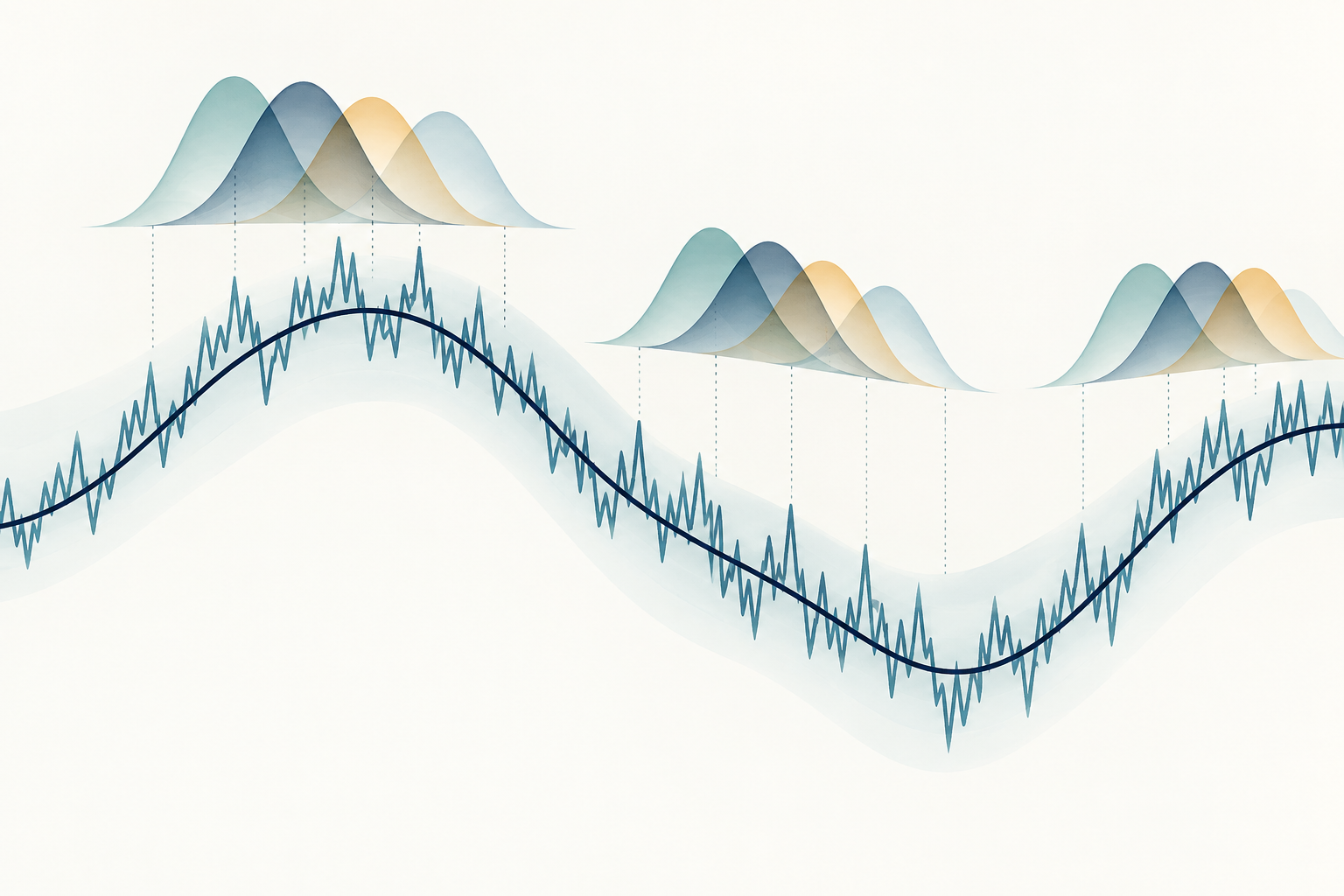
The figure shows a smooth latent path with a jagged observed path and several overlapping tapered windows. It is an explanatory illustration of local pooling, not a sample price record or an empirical filter output.

<!-- learn:illustration --> <!-- Text-free concept: a smooth latent price curve beside a jagged observed path, with overlapping tapered local windows pooling neighboring movements. Conceptual only; not market data, a forecast, or a trading signal. -->

Pre-averaging reduces the influence of fast observation errors, but the squared filtered returns still have a noise contribution. For a regular grid, a common asymptotic-normalizer form of the univariate estimator is

\[ \widehat{IV}_{PA} =\frac{1}{k_n\psi_2}\sum_{i=0}^{n-k_n+1}\bar r_i^2 -\frac{\psi_1}{2\psi_2 k_n^2}\sum_{i=1}^{n}r_i^2, \]

where the weight constants are

\[ \psi_1=\int_0^1 \{g'(u)\}^2\,du, \qquad \psi_2=\int_0^1 g(u)^2\,du. \]

The first term rescales the pre-averaged squared returns toward integrated variance. The second term estimates and subtracts the leading effect of observation noise under the model. It is not an estimate of every noise realization and cannot correct a wrong price field, a bad timestamp, or an outlier. The exact finite-sample formula may use discrete versions of \(\psi_1\) and \(\psi_2\), endpoint adjustments, and a particular return-index convention. Those details must be reported and kept consistent.

The correction can make a finite-sample estimate small or negative. That does not mean an asset had negative physical variance; it means the chosen correction exceeded the first term in that sample. Do not silently set a negative estimate to zero. Report the raw calculation and any separate truncation rule, because truncation changes the estimator and can affect downstream averages or inference.

The window \(k_n\) controls how much smoothing is applied. If it is too short, filtered returns retain more high-frequency noise. If it is too long, local price variation is averaged across a wider time span and fewer windows contribute, increasing other forms of estimation error. The weights and window length work together; a \(k_n\) value is not meaningful without the weight function and sampling interval.

Under the classical balanced design with a fixed time span and \(n\) increasingly frequent observations, the window grows on the order of \(\sqrt n\), often written \(k_n\sim\theta\sqrt n\) for a positive tuning constant \(\theta\). The corresponding estimator can converge at rate \(n^{1/4}\), or have estimation error of order \(n^{-1/4}\), under the paper’s assumptions. This is slower than the noise-free \(n^{1/2}\) rate and is the optimal rate in the baseline noisy setting studied by the authors; it is not a promise about every market dataset.

The constant \(\theta\), weight function, and any plug-in selection procedure affect finite-sample bias and variance. A data-driven choice can depend on noise and volatility estimates that are themselves uncertain. Analysts should show sensitivity across defensible window settings, explain the sampling clock and session boundaries, and avoid selecting a window after seeing which value best supports a preferred conclusion.

Take six hypothetical observed returns, in basis points:

\[ (r_1,\ldots,r_6)=(1,0,1,0,1,0)\ \mathrm{bp}. \]

Use a triangular weight \(g(u)=\min(u,1-u)\) and a deliberately short window \(k=3\). The two nonzero grid weights are \(g(1/3)=g(2/3)=1/3\). For a finite-grid arithmetic illustration, define

\[ \psi_{2,k}=\frac{1}{k}\sum_{j=1}^{k-1}g(j/k)^2=\frac{2}{27}, \qquad \psi_{1,k}=k\sum_{j=1}^{k}\{g(j/k)-g((j-1)/k)\}^2=\frac{2}{3}. \]

There are \(n-k+2=5\) overlapping windows under the index convention above. Each one combines a neighboring \(1\) bp and \(0\) bp return, so \(\bar r_i=(1/3)(1+0)=1/3\) bp and

\[ \sum_i\bar r_i^2=5\left(\frac13\right)^2=\frac59\ \mathrm{bp}^2, \qquad \sum_{i=1}^{6}r_i^2=3\ \mathrm{bp}^2. \]

Using the corresponding finite-grid normalization gives

\[ \widehat{IV}_{PA} =\frac{1}{3(2/27)}\left(\frac59\right) -\frac{2/3}{2(2/27)3^2}(3) =2.5-1.5=1\ \mathrm{bp}^2. \]

This example checks the arithmetic and units; six returns and a three-return-scale window are far too small to support the asymptotic approximation. The returns were chosen for transparency and are not market data, a simulated noise process, or evidence that the estimate recovered a hidden integrated variance. No standard error or forecast is calculated.

The standard derivation is designed for a continuous efficient-price process observed frequently with additive noise under regularity conditions. A centered independent-noise example is a helpful starting point, but dependence between noise and price, serially correlated errors, time-varying noise, irregular observation times, or endogenous sampling may require a modified estimator or a theory tailored to that setting. Aït-Sahalia, Mykland, and Zhang study integrated-volatility estimation with dependent microstructure noise; their paper is one reason not to treat the iid-noise formula as universal.

Jumps raise a separate target question. If the object is quadratic variation, jump squares belong to that quantity; if the object is continuous integrated variance, a standard pre-averaging estimate does not automatically separate jumps. Jump-robust truncation or another construction needs its own assumptions and tuning. A large isolated print can also dominate several overlapping windows, so data validation and outlier treatment remain necessary.

Pre-averaging is also not by itself a complete multivariate or asynchronous-data solution. Christensen, Kinnebrock, and Podolskij develop pre-averaging covariance methods and a noise-robust Hayashi–Yoshida extension for non-synchronous observations in their study. Those constructions address additional design issues; applying a univariate formula asset by asset does not automatically yield a valid covariance matrix or solve mismatched timestamps.

These estimators target related high-frequency variation problems, but they organize the information differently. Two-scale realized volatility averages estimates from shifted sparse sampling grids and subtracts a scaled fine-grid estimate to correct leading noise bias. Pre-averaging first filters short overlapping return windows with a smooth weight, squares those filtered returns, and applies a matching correction. The original two-scale paper provides the basis for that separate construction.

A realized kernel starts from the squared-return sum and adds weighted return autocovariances across lags. It controls the lag range with a kernel bandwidth. Pre-averaging instead modifies local returns before forming squares. Both use weights and tuning choices, but their formulas, normalizations, and assumptions are not interchangeable. See the realized-kernel guide for its lag-based construction and bandwidth discussion.

The choice among methods should follow the data and the quantity needed, not the estimator name. Compare the sampling design, noise model, treatment of endpoints, jump target, and finite-sample behavior. A method’s asymptotic robustness does not guarantee that it is best for sparse assets, a short session, changing noise, or an irregular data feed. The two-scale guide explains its own scale and correction choices.

A reproducible result names the asset and input price field, time interval, sampling frequency, timestamp and session rules, return units, weight function, window length, normalization, endpoint convention, and noise assumptions. If the estimate is used for inference, report the variance estimator or confidence procedure and the assumptions needed for it. A sensitivity table across reasonable windows can reveal whether the conclusion depends on one tuning choice.

Integrated variance is measured over the completed observation interval. Taking a square root expresses a volatility scale over that same interval; annualizing it adds a time convention and does not make the number a forecast. Forecasting a later horizon requires a separate predictive model and out-of-sample evaluation. The realized-volatility calculation guide explains the basic realized-variance benchmark, while the quadratic-variation guide distinguishes path variation from the continuous integrated-variance target.

An estimate does not establish why the price moved, identify a profitable strategy, or guarantee executable risk measurement. Trading costs, liquidity, jumps, volatility dynamics, and estimator uncertainty remain separate questions. Pre-averaging is a statistical measurement tool whose value depends on a transparent match between its assumptions and the observed data.