

Hasbrouck Information Share: Measuring Price Discovery Across Markets
Learn how Hasbrouck information share uses a cointegrated price system and VECM innovations to compare price discovery across markets, including Cholesky-order bounds.
In this guidePrice discovery asks where new information enters a shared price
Short summary
Hasbrouck information share estimates how much each market's price innovations contribute to changes in a common permanent price when the same or closely linked asset trades in more than one venue. It is a variance decomposition built from a cointegrated price system, not a direct count of where news originated. When venue innovations are correlated, Cholesky ordering affects the allocation, so the result should be reported as ordering-sensitive bounds or with an explicit identification choice.
Price discovery asks where new information enters a shared price
The same security can trade in multiple venues, or closely linked instruments can reflect one underlying value. Their observed prices need not match at every instant. A quote may move first in one venue, another venue may react, and both prices may later settle around a common long-run path. Price discovery concerns how new information becomes incorporated into that shared permanent component; it is distinct from trading volume, quoted liquidity, or which venue printed the latest transaction.
Hasbrouck's information share is designed for that question. In his framework, linked market prices share an implicit unobserved efficient price, while each observed price can also contain temporary deviations. A market's share is the proportional contribution of its innovations to the variance of the common efficient-price innovation (Hasbrouck, 1995). The estimate depends on a specified system, sample, and observation design. It does not identify who received information first, establish a causal channel, or show that a venue leads every event.
This distinction matters when a venue has more volume or tighter quotes. Those properties may be associated with price discovery, but information share measures a model-based contribution to permanent price variation. A market can have substantial volume while another market contributes more of the innovations that move the shared long-run price.
A common efficient price requires a cointegrated system
Let p_t contain the observed prices for d venues trading the same asset or economically equivalent claims. The usual microstructure setup treats each price level as nonstationary, often I(1), while long-run arbitrage keeps price differences stationary. With two venues and one common trend, the system has one cointegrating relation, commonly a normalized price difference. More generally, d linked prices with a single shared stochastic trend have cointegration rank d−1.
This is an empirical assumption to examine, not an identity that follows from listing the same ticker on two screens. Prices may differ because of contract terms, currency, funding, dividends, delivery, or a persistent basis. The relationship can also change after a venue migration, fee change, market-structure reform, or data-definition change. If the observed series do not share the assumed long-run relation over the chosen sample, the efficient-price decomposition and its shares do not have the intended interpretation.
Cointegration and error correction connect a stationary long-run relation to a model for short-run price changes (Engle and Granger, 1987). The VECM makes that structure explicit. It separates temporary adjustment around the common price from innovations that can affect the long-run component.
<!-- learn:illustration --> <!-- Text-free concept: two venue price paths fluctuate around one shared, smoother long-run price path, with temporary venue-level deviations. Not market data, a causal diagram, or a forecast. -->
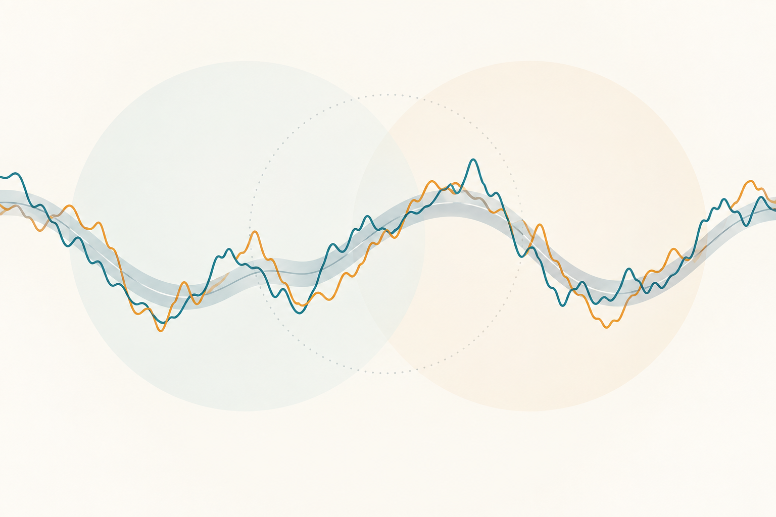
The VECM links venue prices to the common permanent component
For d price series, a VECM can be written as
\[ \Delta p_t=\alpha\beta^{\mathsf T}p_{t-1} +\sum_{j=1}^{q-1}\Gamma_j\Delta p_{t-j}+\varepsilon_t, \qquad \Pi=\alpha\beta^{\mathsf T}. \]
Here β spans the cointegrating relations, α contains the adjustment loadings, Γ_j captures short-run lag dynamics, and ε_t is the vector of reduced-form innovations with covariance matrix Ω. In the common one-efficient-price case, the long-run impact of these innovations can be summarized by a row vector ψ. The increment in the permanent price is
\[ \Delta m_t=\psi\varepsilon_t, \]
up to the model's chosen normalization and deterministic terms. The total variance of that increment is
\[ \operatorname{Var}(\Delta m_t)=\psi\Omega\psi^{\mathsf T}. \]
The vector ψ is obtained from the fitted system's long-run representation; it is not simply the adjustment coefficient α or the cointegrating vector β. Short-run price changes can be large but transitory, while a smaller innovation can matter more for price discovery if its effect remains in the shared permanent component.
The common trend and its normalization must be stated. Multiplying the efficient-price representation by a constant changes the units of ψ and the common-price variance, though normalized information shares remain unchanged. If the system has more than one common stochastic trend, a single scalar efficient price is not enough; the researcher must define which permanent component or linear combination is being decomposed.
Information share decomposes the variance of permanent innovations
If venue innovations are uncorrelated, Ω is diagonal. Each market's contribution to permanent-price variance can then be separated directly:
\[ \operatorname{IS}_i= \frac{\psi_i^2\Omega_{ii}}{\psi\Omega\psi^{\mathsf T}}, \qquad \sum_{i=1}^{d}\operatorname{IS}_i=1. \]
This formula weights a market's long-run impact by the variance of its own innovation. A venue whose price innovation has a larger persistent effect or more innovation variance can receive a larger information share. It is not enough to compare the absolute sizes of VECM adjustment coefficients.
When innovations are contemporaneously correlated, the total variance includes covariance terms. There is no unique way to assign those shared terms to individual venues from Ω alone. Hasbrouck uses a Cholesky factorization Ω=FF^T to form orthogonal innovations. For a selected variable ordering, the share assigned to orthogonal shock i is
\[ \operatorname{IS}_i(F)= \frac{(\psi F)_i^2}{\psi\Omega\psi^{\mathsf T}}. \]
The factorization makes the shocks orthogonal, but its triangular structure gives earlier variables in the ordering a priority in absorbing shared contemporaneous variation. The ordering is an allocation convention for the decomposition, not proof of an economic information hierarchy.
Correlated innovations make the Cholesky ordering visible
If two venue innovations are highly correlated because their prices update within the same sampling interval, the data do not cleanly separate which market's innovation arrived first. A Cholesky decomposition assigns their common movement differently depending on which venue is ordered first. Hasbrouck's procedure reports a lower bound by placing a market last and an upper bound by placing it first, across the relevant orderings.
These bounds answer a more honest question than a single convenient ordering: how much could this market's share vary under the admissible recursive allocations of correlated innovations? Narrow bounds indicate that this particular ordering issue has little effect in the fitted sample. Wide bounds mean the venue-level split is weakly identified by contemporaneous price innovations. A midpoint is sometimes reported as a summary, but it is not a uniquely identified estimate and should not replace the bounds or a stated ordering.
Sampling more frequently may reduce some apparent contemporaneous correlation when one venue updates before another, but it does not guarantee zero correlation. Coarse sampling hides the sequence of price updates; very fine sampling can create stale observations and asynchronous quote problems. Report both the sampling rule and the ordering sensitivity.
A fully hypothetical two-market example shows the bounds
Suppose, purely for illustration, a fitted two-market VECM implies a normalized permanent-price impact vector \(\psi=(0.6,0.4)\). Let the reduced-form innovation covariance matrix be
\[ \Omega= \begin{pmatrix} 1 & 0.8\\ 0.8 & 1 \end{pmatrix}. \]
The innovations have unit variance and correlation 0.8. The total variance of the permanent-price innovation is
\[ \psi\Omega\psi^{\mathsf T} =0.6^2+0.4^2+2(0.6)(0.4)(0.8) =0.904. \]
Order Market A first. A lower-triangular Cholesky factor is
\[ F_A= \begin{pmatrix} 1 & 0\\ 0.8 & 0.6 \end{pmatrix}, \qquad \psi F_A=(0.92,0.24). \]
The resulting shares are A: \(0.92^2/0.904\approx93.6\%\), and B: \(0.24^2/0.904\approx6.4\%\). Reverse the ordering and put B first. The same calculation assigns about 85.7% to B and 14.3% to A. Thus the ordering-based bounds are approximately 14.3%–93.6% for A and 6.4%–85.7% for B. Each ordering sums to 100%; the separate lower bounds or upper bounds across markets are not meant to sum to 100%.
Every value here is hypothetical: the VECM impact vector, unit innovation variances, and 0.8 correlation are chosen only to make the arithmetic reproducible. The example is not a result for any exchange, asset, or sample. Its purpose is to show how correlated innovations can make a seemingly precise market ranking depend heavily on the Cholesky ordering.
Gonzalo–Granger component shares answer a different question
The Gonzalo–Granger decomposition constructs a permanent component as a normalized linear combination of observed prices. In a VECM with adjustment matrix α, the common-factor weights lie in the orthogonal complement of α: a weight vector w satisfies α^T w=0, with a normalization such as the weights summing to one. The resulting common factor does not respond in the long run to the error-correction terms. Gonzalo and Granger developed this permanent–transitory decomposition for cointegrated systems (Gonzalo and Granger, 1995).
Those component weights describe how the common price level is formed from venue prices. Hasbrouck information shares instead measure each venue's contribution to the variance of innovations in the common permanent price. The two can be closely related, but the information share also accounts for the variance of each venue's innovation. De Jong's comparison and Baillie, Booth, Tse, and Zabotina's analysis explain why the measures may look similar when innovations are uncorrelated and diverge when they are correlated or have different variances (de Jong, 200200028-9); Baillie et al., 200200027-7)).
The hypothetical inputs ψ and Ω above do not determine Gonzalo–Granger component weights, which depend on the VECM adjustment matrix α and a stated normalization. No numerical component weight follows from the variance-decomposition inputs alone. This difference is central: component weights construct a permanent price from observed prices, while Hasbrouck information shares decompose variance in its innovation.
Data timing and model choices can change the estimate
The price series must describe comparable claims and be aligned to a defensible clock. Specify whether each observation is a trade price, midpoint, or another quote measure; how you handle locked or crossed quotes, stale prices, auctions, market closures, and out-of-sequence messages; and whether both venues are open during the sample. For futures, document contract rolls and delivery differences. For cross-listed instruments, align currencies, corporate actions, and units before estimating the VECM.
Asynchronous observations are a central concern. If one venue updates at 10:00:00.100 and another at 10:00:00.700, a one-second sampling grid can make a sequential response look simultaneous; a coarser grid can blur it further. A very fine grid may instead carry forward stale prices, creating artificial lead–lag patterns. Report the sampling frequency, synchronization rule, quote filters, and sensitivity to reasonable alternatives. Shorter intervals can reduce aggregation-induced correlation, but they do not eliminate true common shocks, simultaneous updates, or timestamp error.
The share also depends on lag order, deterministic terms, sample endpoints, and structural stability. Too few lags can leave serial dependence in VECM innovations; too many can increase estimation noise. A venue rule change or a shift in trading hours can change the adjustment process. Use residual diagnostics and uncertainty estimates, and consider a bootstrap that re-estimates the full VECM and share bounds. Do not treat a small standard error conditional on one specification as covering uncertainty over model and data choices.
An information share is not a causal ranking or trade signal
An information share quantifies how innovations from each modeled venue contribute to estimated permanent-price variance under a particular VECM and orthogonalization. A high share does not prove that the venue created the news, that it moves first for every event, or that it predicts the next return. Common information can reach venues nearly simultaneously, while market frictions and observation timing affect the measured split.
It is also not a direct measure of market quality. A venue can contribute to the common price while having a wide spread, shallow displayed depth, or high execution costs. Conversely, a venue can offer low-cost liquidity while contributing less to the permanent-price innovation in the chosen sample. The Roll spread estimator estimates a different object from return autocovariance, and order-flow imbalance summarizes displayed queue changes rather than long-run innovation variance.
For a trading claim, the information-share analysis must be part of a pre-specified, out-of-sample strategy test that includes fees, bid–ask spread, latency, slippage, market impact, and venue access. The Engle–Granger guide explains the single-equation cointegration alternative, while the Johansen rank guide covers system cointegration rank. Neither cointegration nor a high information share establishes a profitable rule.
Common questions
Q1Do information shares always sum to 100%?
For a given orthogonalization and ordering, the normalized shares across the modeled markets sum to 100%. If innovations are correlated, the market-specific lower bounds or upper bounds are calculated under different orderings and should not be added across venues.
Q2Does the venue with the highest information share always lead price changes?
No. The estimate summarizes a sample-level variance contribution under a VECM. It does not show that the venue updates first for every event or causes the other venues to move.
Q3Why report a range instead of one information share?
When venue innovations are correlated, a unique allocation of their shared variance is unavailable without an additional ordering or identification assumption. Hasbrouck bounds show how the result changes when each venue is placed first or last.
Q4Can a high information share support a profitable trading strategy?
Not by itself. It does not provide an entry rule, predict the next return, or include execution costs. A complete strategy needs separate chronological out-of-sample testing with venue-specific fees, spread, latency, slippage, and impact.
Sources and further reading
Report an issue
We’ll prepare an email with this article link. Mark receives the report only after you send it
Quick check
Read the guide? Check yourself with 3 questions
Question 01
What does Hasbrouck information share measure?
Choose an answer to see the explanation
Options glossary
A call or put whose strike is near the underlying price; it has little intrinsic value and often substantial sensitivity to time and volatility.
Read the deeper guideCall optionA contract that gives its holder the right, but not the obligation, to buy the underlying at the strike before or at expiration under the contract terms.
Read the deeper guidePut optionA contract that gives its holder the right, but not the obligation, to sell the underlying at the strike before or at expiration under the contract terms.
Read the deeper guide