

Fama–MacBeth Regression: Two-Pass Risk Premiums Explained
Follow the two-pass Fama–MacBeth procedure from time-series beta estimates to date-by-date cross-sectional risk prices, then separate its standard error, Shanken adjustment, and HAC inference.
In this guideIt estimates prices for exposure, not one time-series beta
Short summary
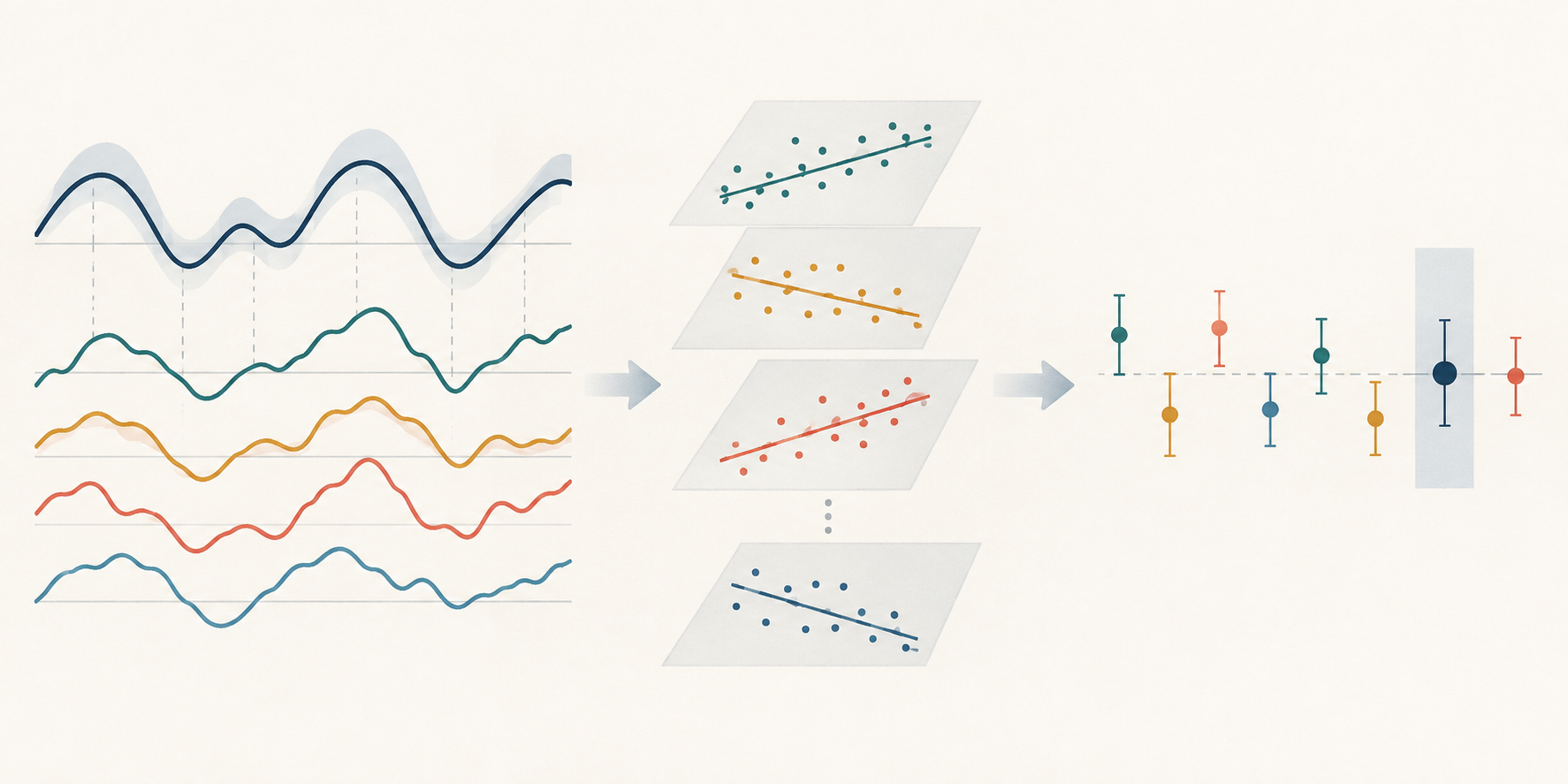
A Fama–MacBeth procedure estimates each test asset’s factor exposure from its time series, regresses returns across assets on those estimated exposures at each date, and averages the resulting risk-price slopes over time. The time series of slopes supplies the usual uncertainty calculation. That second-pass standard error does not automatically account for estimated betas, serial dependence, or a misspecified pricing model, and a significant average risk price is not a trading-profit estimate.
It estimates prices for exposure, not one time-series beta
A factor beta and a factor risk price answer different questions. A beta describes how an asset’s return has moved with a factor in the first-pass time-series regression. A risk-price coefficient, often written \(\lambda\), describes how returns differ across assets with different estimated betas in a second-pass cross-section. The Fama–MacBeth procedure produces a risk-price estimate for each date and then summarizes those estimates through time.
That design is useful when the research question concerns whether exposure to a proposed risk factor is associated with average returns across a chosen set of stocks or portfolios. It is a statistical asset-pricing procedure, not a causal design. Nor does it by itself specify a portfolio that could have been traded using information available at the time.
The original Fama and MacBeth study applied repeated cross-sectional risk-return regressions to NYSE stocks. Later work, including Fama and French’s empirical tests, made month-by-month cross-sectional slopes a familiar way to estimate and test average risk prices. The procedure is best understood as two linked estimation problems, with separate assumptions in each pass.
First pass: estimate each test asset’s exposure
For each asset or test portfolio \(i\), estimate a time-series regression such as
\[ r^{e}_{i,t} = \alpha_i + \boldsymbol{\beta}_i^\top \mathbf{f}_t + \varepsilon_{i,t}, \]
where \(r^{e}_{i,t}\) is the asset’s excess return, \(\mathbf{f}_t\) is the vector of factor returns at date \(t\), and \(\boldsymbol{\beta}_i\) is the exposure vector. The fitted \(\hat{\boldsymbol{\beta}}_i\) becomes an explanatory variable in the second pass. A market-only example has one beta; a multi-factor example has one estimated loading per factor.
The first pass needs enough time-series variation in the factors to estimate those slopes. A long window may provide more observations but mix different market regimes. A short window may reflect recent exposure but leave beta estimates noisy. The researcher should state the return frequency, sample dates, factor construction, missing-data rules, intercept treatment, and estimation window.
This is not a universal instruction to estimate every beta on the full sample. In an ex-post asset-pricing test, full-sample beta estimates may describe the sample under study. In a historical trading simulation, using a beta estimated with future observations would leak information. That use instead needs a point-in-time beta estimate built from data available before each simulated decision.
Second pass: price exposures in each date’s cross-section
At each date \(t\), regress that date’s test-asset returns on the first-pass betas:
\[ r^{e}_{i,t} = \lambda_{0,t} + \hat{\boldsymbol{\beta}}_i^\top \boldsymbol{\lambda}_t + \eta_{i,t}. \]
Here \(\boldsymbol{\lambda}_t\) contains the date-specific prices of risk. With one factor, the cross-sectional slope \(\lambda_t\) measures the return difference associated with one unit of estimated beta in that date’s cross-section. The intercept \(\lambda_{0,t}\) is a separate cross-sectional intercept. Whether it should be estimated freely, constrained, or interpreted as a zero-beta return depends on the tested model and on whether returns are raw or excess returns.
The second regression is across assets at one date; it is not another time-series regression. Its fit depends on the number and composition of test assets, the spread of their estimated betas, and the correlation among those betas. If betas barely differ across assets, the cross-section has little leverage to distinguish one price of risk from another. Adding many nearly identical assets cannot create exposure variation that is not there.
Repeating this regression gives a series \(\hat{\boldsymbol{\lambda}}_1,\ldots,\hat{\boldsymbol{\lambda}}_T\). The Fama–MacBeth estimate for factor \(k\) is the time average
\[ \bar{\lambda}_k = \frac{1}{T}\sum_{t=1}^{T}\hat{\lambda}_{k,t}. \]
The average is in the same return units and frequency as the second-pass returns. If the cross-sections are weighted, dates are missing, or the asset universe changes, those choices affect what this average represents and should be reported.
A worked example separates one month from the average
Suppose three test portfolios have first-pass market beta estimates of \(0.5\), \(1.0\), and \(1.5\). In one hypothetical month, their excess returns are \(0.3\%\), \(0.8\%\), and \(1.3\%\). These three points lie on
\[ r^{e}_{i,t} = -0.2\% + 1.0\%\times\hat{\beta}_{i}. \]
For that month, the estimated slope is \(1.0\) percentage point per beta unit and the intercept is \(-0.2\%\). This exact fit is deliberately small and illustrative; it does not establish that the market beta is priced, and three points do not provide a useful empirical test.
Now imagine the second-pass slope is estimated in six separate months and equals \(0.8\%\), \(-0.4\%\), \(1.0\%\), \(-0.2\%\), \(0.6\%\), and \(0.0\%\) per beta unit. Their arithmetic mean is
\[ (0.8 - 0.4 + 1.0 - 0.2 + 0.6 + 0.0)/6 = 0.3\%\text{ per month}. \]
The first month’s slope is not the final Fama–MacBeth estimate. The estimate is the average across the six date-specific slopes. The negative months remain in the calculation; selecting only positive months would change the estimand and introduce another selection step. These made-up inputs demonstrate the arithmetic only, not a market result or a claim that a factor predicts returns.
The usual standard error uses time as its inferential dimension
In the simplest calculation, take the sample standard deviation \(s_\lambda\) of the \(T\) monthly slope estimates and divide by \(\sqrt{T}\):
\[ \operatorname{SE}(\bar{\lambda}) = \frac{s_\lambda}{\sqrt{T}}. \]
The corresponding t-statistic divides the estimated mean slope by that standard error. This calculation treats time as the repeated dimension for estimating uncertainty in the average risk price. The number of assets \(N\) determines how well each monthly cross-section can estimate a slope; it does not replace \(T\) in the standard error of the time average.
For the six illustrative slopes above, their sample standard deviation is about \(0.576\) percentage point per month. Dividing by \(\sqrt{6}\) gives a conventional standard error of about \(0.235\) percentage point; \(0.3/0.235\) is about \(1.28\). Six observations are far too few for this to be a reliable significance assessment. The calculation only shows why a positive average and a precisely estimated average are not the same claim.
The usual standard error also relies on conditions for the time series of slopes. If estimates are serially dependent, an independent-observation standard error can misstate the uncertainty. If the sample is short or the asset mix changes, asymptotic t-statistics can be especially fragile. Report the length and frequency of the \(\lambda_t\) series, not only the cross-sectional asset count.
Fama–MacBeth and pooled OLS are not always different point estimates
It is common to contrast “Fama–MacBeth” with “pooled panel regression” as if the procedures must produce different slopes. There is an important special case. If the same assets appear at every date, the beta regressors are fixed across dates, and every monthly cross-section uses the same ordinary least-squares design, averaging the date-specific OLS coefficients gives the same common-slope coefficient as pooled OLS. Both are summarizing the same balanced set of cross-sectional regressions.
The equality can break when the asset set or weights change across dates, the betas vary through time, the panel is unbalanced, the regressions use different controls, or the pooled model imposes additional restrictions. In those cases the procedures can weight dates or observations differently and answer different sample questions. One should not choose a method by the name alone; write down the exact design matrix, weighting scheme, and target coefficient.
Even when point estimates coincide, the uncertainty calculation may not. Fama–MacBeth inference uses the time variation of the cross-sectional slopes. A pooled regression needs a covariance estimator that matches its panel error structure. Clustering by date or asset, a two-way covariance estimate, or a time-series HAC estimate each rests on different assumptions; none is made correct simply by calling the model pooled or Fama–MacBeth.
Estimated betas and HAC address separate uncertainty
The second pass treats \(\hat{\boldsymbol{\beta}}_i\) as if it were known, although it came from an estimated first-pass regression. Error in a generated regressor can affect the risk-price estimate and its uncertainty. Shanken’s analysis derives an adjustment for beta-pricing inference under a specified asset-pricing setup; it is not a universal multiplier that repairs every two-pass design. Later work studies the large-sample behavior and alternative estimators under different conditions. State the correction or inference method used and the assumptions that make it relevant.
Serial correlation in \(\hat{\lambda}_{k,t}\) is a different problem. For example, overlapping multi-month returns can make adjacent second-pass slopes share return observations. A heteroskedasticity-and-autocorrelation-consistent estimate, such as a Newey–West covariance estimate, adjusts the estimated variance of the time average for serial dependence up to a selected lag window. It does not put the first-pass beta estimation error back into the second pass, fix factor misspecification, or cure look-ahead bias. Conversely, a Shanken adjustment is not a substitute for checking dependence in the lambda series.
Jagannathan and Wang and Shanken and Zhou analyze the properties of beta-pricing procedures under particular model and sampling conditions. Their results are a reason to describe the actual two-pass design instead of repeating a blanket rule that ordinary Fama–MacBeth errors are always too small or always valid. Report whether betas are estimated once or updated, how the lambda series’ dependence is handled, whether a generated-beta correction is used, and why that choice matches the question.
A significant average risk price is not a trading-profit estimate
A positive, statistically distinguishable mean \(\lambda\) says that, under the selected test-asset universe, factor definition, beta estimates, and inference procedure, assets with greater estimated exposure had higher average returns in the sample. It does not show that an investor could earn that spread after costs, that the factor is a causal source of return, or that the pricing model is correct.
The result can change when the factor set, sample period, portfolio construction, beta window, test assets, or weighting scheme changes. Searching across many factors, sample cuts, and specifications adds a multiple-testing problem. A test of one estimated risk price also does not summarize joint pricing errors for every asset. State whether a result is a conditional association, a model-based pricing test, or an out-of-sample forecast; do not use those labels interchangeably.
For a live or simulated strategy, exposures and portfolio weights must be formed using only information then available. The strategy also needs executable entry prices, turnover, trading costs, financing, capacity, and a rebalancing rule. The factor beta is an exposure estimate; the average \(\lambda\) is not the return of a portfolio that automatically earns that beta premium. For the surrounding concepts, see the guides to factor loadings and factor models, robust standard errors and HAC, and rank information coefficients.
Report the design so another researcher can reproduce it
An interpretable result identifies the test assets, factor returns, risk-free series if used, return units, date frequency, and sample period. It also records how each beta was estimated, whether the first-pass window overlaps the second-pass test period, which assets enter each date, how missing returns and changing membership are handled, whether cross-sections are weighted, and whether an intercept is included or constrained.
For inference, report the full number of date-specific slopes \(T\), their time-series mean and dispersion, the standard-error estimator, any HAC bandwidth, any beta-estimation correction, and any finite-sample choices. Show beta dispersion and cross-sectional fit as well as t-statistics; a large asset count cannot compensate for almost identical exposures. Compare reasonable alternative windows, factor definitions, and test-asset constructions without selecting the version that happens to give the smallest p-value.
The original method and applications provide examples, not a guarantee that every modern dataset satisfies their assumptions. Fama and MacBeth’s 1973 paper, Fama and French’s 1992 cross-sectional tests, Shanken’s beta-pricing analysis, Jagannathan and Wang’s asymptotic analysis, Shanken and Zhou’s comparison of beta-pricing estimators, and Newey and West’s HAC covariance method address different pieces of the design. Read the assumptions alongside the reported coefficient.
Common questions
Q1Is a Fama–MacBeth regression a causal test?
No. It estimates an association between estimated exposures and returns under a selected pricing model and test-asset design. Causal interpretation needs a separate identification argument.
Q2Does adding more assets always make the risk-price estimate more precise?
No. More assets can improve a date’s cross-section, but precision also depends on how much their betas vary, how accurately those betas were estimated, and how many dates contribute to the average.
Q3When should I use a HAC standard error?
Consider it when the date-specific risk-price series may be heteroskedastic or serially dependent, such as with overlapping returns. State the lag window and remember that HAC does not correct first-pass beta error.
Sources and further reading
Report an issue
We’ll prepare an email with this article link. Mark receives the report only after you send it
Quick check
Read the guide? Check yourself with 3 questions
Question 01
In the standard two-pass procedure, what does the second-pass slope at date t estimate?
Choose an answer to see the explanation
Options glossary
A model decomposing asset returns into exposure to a small set of common factors and an asset-specific residual.
Read the deeper guideHeteroskedasticityVariation in the conditional error variance across regressor values or states, invalidating an equal-variance covariance formula.
Read the deeper guideStochastic discount factorA random variable that weights future payoffs by time and state value to produce today's price; asset returns satisfy its pricing moment condition.
Read the deeper guide