Engle–Granger Cointegration Test: Residual और Error Correction

दो trending series साझा stochastic trend के कारण संबंधित दिख सकते हैं। Cointegration इससे अधिक विशिष्ट बात है: यदि अलग-अलग series integrated of order one, I(1), हैं, तो उनके किसी खास weighted combination का stationary, I(0), होना संभव है। चुने हुए model में यह combination long-run equilibrium error है। यह बिना सीमा भटकने के बजाय स्थिर distribution के आसपास बदलता है।

Engle–Granger two-step procedure एक equation से इस दावे की जाँच करता है। पहले step में levels पर long-run relation estimate होता है। दूसरे में estimated residual में unit root की जाँच होती है। First-stage equation में किस variable को बाईं तरफ रखें, यह चुनना पड़ता है; इसलिए finite sample में test का नतीजा दिशा पर निर्भर हो सकता है। यहाँ classical two-variable setup है। कई cointegrating relations संभव हों तो यह system method का विकल्प नहीं है।

आम setup मानता है कि component variables I(1) हैं: चुनी हुई specification में levels nonstationary और first differences stationary हैं। Unit-root tests पूर्ण नहीं होते, खासकर छोटे sample या structural break के आसपास। इसलिए integration-order जाँच को यांत्रिक pass/fail शर्त नहीं, बल्कि evidence मानें। I(0) series को I(1) series के साथ मिलाना यहाँ बताए classical I(1) cointegration case में नहीं आता।

Data-generating question के आधार पर तय करें कि long-run equation में intercept, deterministic trend, या दोनों में से कोई नहीं होगा। उदाहरण के लिए, log asset prices के spread में intercept हो सकता है, पर deterministic trend नहीं; किसी economic aggregate में trend ज़रूरी हो सकता है। Deterministic terms अनुमानित equilibrium और residual-test distribution दोनों को बदलते हैं। छोटा p-value देखने के बाद इन्हें चुनने से test समझना कठिन होता है।

दो level series \(y_t\) और \(x_t\) के लिए एक सरल first-stage equation है:

\[ y_t = a + \beta x_t + u_t. \]

मान्य assumptions के तहत ordinary least squares से \(a\) और \(\beta\) estimate करें, फिर \(\hat u_t = y_t-\hat a-\hat\beta x_t\) सहेजें। इस specification में series cointegrated हों तो अलग-अलग levels nonstationary होने पर भी fitted combination stationary होना चाहिए।

Finance के उदाहरण में \(y_t\) और \(x_t\) एक ही frequency पर देखे गए दो assets के log total-return indexes हो सकते हैं। \(\hat\beta\) fitted long-run combination तय करता है; यह अपने-आप dollar-neutral या low-risk portfolio weight नहीं होता। Left-hand variable, sample, dividends का treatment, currency या trend specification बदलने से estimate और residual बदल सकते हैं। Equation का economic meaning स्पष्ट रखें।

Augmented Dickey–Fuller प्रकार की residual regression को इस तरह लिख सकते हैं:

\[ \Delta\hat u_t = \rho\hat u_{t-1} + \sum_{j=1}^{q}\phi_j\Delta\hat u_{t-j} + e_t. \]

No-cointegration null hypothesis का अर्थ है कि residual में unit root है; alternative यह कि fitted residual stationary है। इस सरल notation में पर्याप्त negative residual-test statistic null के विरुद्ध evidence देता है। Lag terms residual की serial dependence दर्शाने में मदद करते हैं, इसलिए lag order और residual diagnostics महत्वपूर्ण हैं। यह निर्णय first-stage intercept या trend चुनने से अलग है, जो cointegration critical-value case तय करता है। Augmenting lags बहुत कम हों तो serial correlation बच सकती है। Agiakloglou और Newbold की चर्चा के अनुसार, lag order चुनने का तरीका बताएँ और उचित विकल्प भी जाँचें।

Residual पहले step में estimate होता है, इसलिए null के तहत उसका distribution बदल जाता है। इस statistic की तुलना सामान्य Dickey–Fuller critical values या generic ADF p-value से न करें। चुने हुए deterministic terms, variables की संख्या और sample size के अनुरूप Engle–Granger residual-test critical values या p-values लें। Phillips और Ouliaris ने residual-based tests की asymptotic theory विकसित की; MacKinnon ने आम specifications के लिए response-surface critical values दिए। इसलिए residual-test statistic का संख्यात्मक मान समान होने पर भी, first-stage deterministic terms या explanatory variables की संख्या बदलने से तुलना के लिए reference critical value अलग हो सकती है।

मान लें कि एक शोधकर्ता तय monthly sample में दो log-price indexes देखता है। बताई गई unit-root specifications के तहत दोनों I(1) लगते हैं। First-stage regression में intercept है और उससे fitted residual मिलता है। Residual statistic को सामान्य ADF table से नहीं, उस deterministic setup और sample के अनुकूल Engle–Granger distribution से आँका जाता है।

मान लें matching test का p-value, शोधकर्ता की पहले से तय 5% सीमा से कम है। शोधकर्ता इस specification के लिए no-cointegration null को reject करता है और estimated combination के stationary होने का evidence पाता है। यह निष्कर्ष sample, lag choice, deterministic terms और integration assumptions पर निर्भर है। इससे यह साबित नहीं होता कि हर asset pair संबंधित है, relation sample के बाहर कायम रहेगा या fitted residual लाभदायक entry signal देगा। p-value 5% से ऊपर हो तो सही अर्थ है “इस specification में no-cointegration को reject नहीं किया गया,” न कि “series असंबंधित साबित हुईं।”

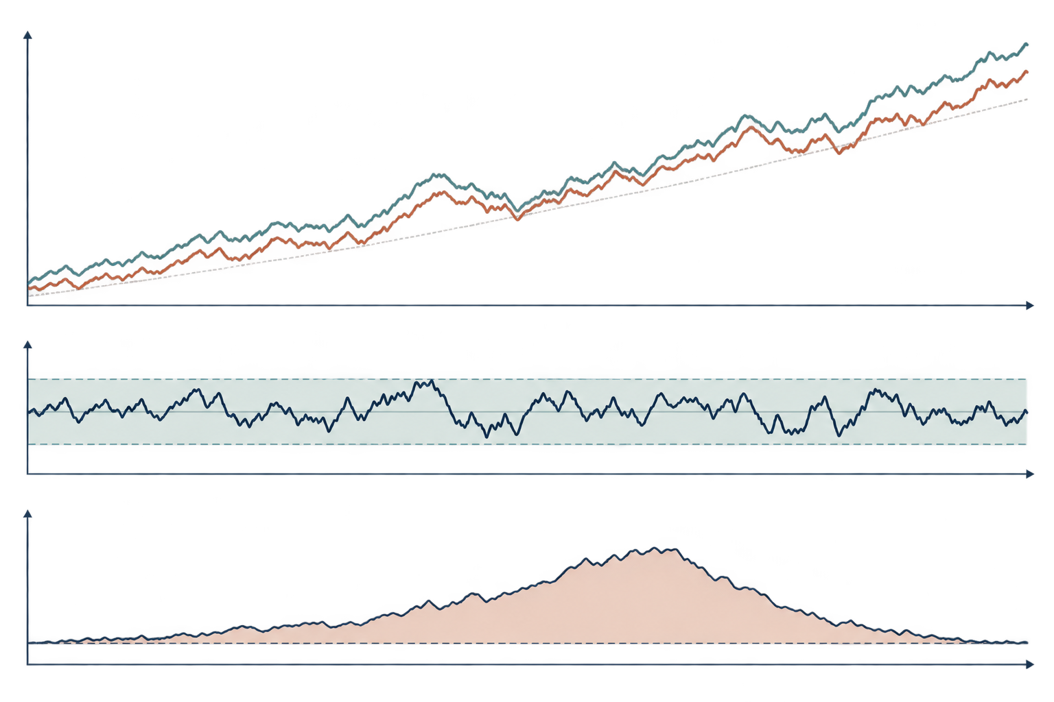
नीचे का चित्र अवधारणात्मक है: साझा stochastic trend के साथ bounded residual हो सकता है और fitted relation से deviation बाद में कम हो सकता है। इसमें मापी गई series नहीं हैं और यह नहीं कहता कि adjustment हमेशा अनुमानित गति से होगा।

Long-run relation के समर्थन में evidence हो तो error-correction model short-run changes को पिछले period के equilibrium error से जोड़ सकता है। यदि \(\hat u_{t-1}=y_{t-1}-\hat a-\hat\beta x_{t-1}\), तो एक उदाहरण है:

\[ \Delta y_t = c + \lambda\hat u_{t-1} + \sum_{i=1}^{r}\phi_i\Delta y_{t-i} + \sum_{j=0}^{s}\theta_j\Delta x_{t-j} + \epsilon_t. \]

यहाँ \(\lambda\) इस parameterization में \(y_t\) का adjustment coefficient है। यदि \(y\) fitted relation से ऊपर है और \(\lambda<0\), तो बाकी सब समान रहने पर error-correction term \(y\) में गिरावट की दिशा में योगदान देता है। यह sign reading \(\hat u=y-\hat a-\hat\beta x\) की परिभाषा पर निर्भर है; residual convention उलटने से coefficient का sign भी उलट जाता है। Short-run coefficients अतिरिक्त conditional responses बताते हैं। दूसरा variable भी adjust कर सकता है; cointegration अकेले यह नहीं बताता कि कौन-सा market या economic variable adjustment करेगा।

\(\lambda\) को सीधे “हर महीने spread का इतना प्रतिशत बंद होता है” न कहें, जब तक model में सचमुच ऐसा सरल dynamic form न हो। Lagged changes, कई adjusting variables, nonlinear responses और breaks पूरी राह को प्रभावित करते हैं। Stable long-run relation कोई structural causal mechanism नहीं है; adjustment coefficient चुने हुए model और information set के संदर्भ में ही समझें।

Engle–Granger single-equation setup एक प्रस्तावित long-run combination test कर सकता है, जिसमें dependent variable और कई regressors हो सकते हैं। दो I(1) variables के लिए अधिकतम cointegration rank एक है; बड़े system में कई cointegrating vectors हो सकते हैं। एक residual test पूरे system का rank नहीं तय करता। Johansen procedure अपनी VAR और deterministic-term assumptions के तहत rank के प्रश्न के लिए बनाया गया है।

Finite sample में first-stage normalization भी मायने रखता है। Long-run relation अवधारणा में एक combination है, लेकिन \(y\) को \(x\) पर regress करने का numerical परिणाम आम तौर पर \(x\) को \(y\) पर regress करने के बराबर नहीं होता। साफ़ economic reason से normalization चुनें और report करें। Equation उलटने पर नतीजा बदले तो अनुकूल परिणाम चुनने के बजाय sensitivity बताएँ।

छोटे sample में test की power कम हो सकती है। Lag choice, deterministic terms, outliers और structural breaks भी नतीजे बदल सकते हैं। Long-run relation में break होने पर पहले stationary combination पूरे sample में अस्थिर दिख सकता है। एक rejection, बनाए रखी गई specification के तहत evidence है—relation हमेशा रहेगा इसका प्रमाण नहीं।

Trading application में fitted residual को spread कहा जा सकता है, लेकिन नाम से executable portfolio तय नहीं होता। Log prices से बना spread dollar-valued position से अलग है; price-only series total-return series से अलग है। Regression coefficient बदल सकता है, और residual stationary estimate होने पर भी entry threshold, holding period, stop या position size अपने-आप नहीं मिलते।

Long-run relation हर decision date तक उपलब्ध data से ही estimate करें। पूरे backtest sample का hedge coefficient निकालकर पुराने समय में trade करने से signal में future observation leak होगा। Chronological formation और evaluation windows रखें; dividends, splits, borrow availability, financing, bid–ask spread, market impact और rebalancing शामिल करें। Diagnostics break दिखाएँ तो क्या करेंगे, यह तय करें। कई pairs और windows खोजना selection bias लाता है, जिसे cointegration test ठीक नहीं करता।

व्यावहारिक प्रश्न सिर्फ यह नहीं कि residual test reject करता है या नहीं। पूछें कि economic link के बने रहने का कारण है या नहीं, वह पारदर्शी stability check में टिकता है या नहीं, और uncertainty व costs के बाद कोई implementable rule बचता है या नहीं। Cointegration model को जानकारी दे सकता है; convergence, hedge effectiveness या returns की guarantee नहीं।

Variables, transformations, frequency, sample dates, integration evidence और first-stage normalization बताएँ। Intercept या trend, residual-test type, lag-selection rule, test statistic और cointegration-specific critical values या p-values का source दर्ज करें। तर्कसंगत वैकल्पिक lag या sample window पर sensitivity दिखाएँ और break analysis हुआ या नहीं बताएँ।

Error-correction model estimate करने पर lagged disequilibrium term और sign convention परिभाषित करें, कौन-से variables adjust कर सकते हैं बताएँ, और short-run coefficients को long-run relation से अलग रखें। Trading study में chronological splits, pair-selection rules, costs, financing, borrow assumptions और failure handling बताएँ। इन ब्योरे से reproducible test और केवल convergence जैसा दिखने वाला chart अलग होते हैं।

Engle और Granger का cointegration, estimation और testing पर मूल paper, cointegration और error correction के संबंध को विकसित करता है। Phillips और Ouliaris ने residual-based cointegration tests की asymptotic theory दी। MacKinnon का critical-value अध्ययन sample size और test specification पर निर्भर response-surface values समझाता है। Agiakloglou और Newbold ने augmented Dickey–Fuller test की lag structure90022-Q) का अध्ययन किया। कई संभावित relations वाले system के लिए Johansen का cointegrating-vector analysis90041-3) देखें। संबंधित मार्गदर्शिकाएँ हैं pairs trading में cointegration और correlation, finance में stationarity, unit roots और mean reversion, और impulse responses के लिए local projections।