CAViaR Explained: Conditional Autoregressive Value at Risk

Let \(L_t=-r_t\) denote portfolio loss, so a loss is positive and a gain is negative. For confidence level \(\alpha\), a one-step VaR forecast is the conditional upper quantile \[ v_t^\alpha=Q_\alpha(L_t\mid\mathcal F_{t-1}), \] where \(\mathcal F_{t-1}\) contains information available before period \(t\)'s loss is observed. At \(\alpha=0.99\), the target is a threshold that should be exceeded by roughly \(1-\alpha=1\%\) of future losses when the conditional quantile is correctly specified. The realized loss can exceed VaR by any amount; VaR is not a maximum-loss limit.

CAViaR, short for Conditional Autoregressive Value at Risk, specifies how this quantile changes over time using a recursion. Instead of estimating the entire conditional distribution and extracting one tail point afterward, it models that point directly. Engle and Manganelli introduced this class and estimated its parameters using regression quantiles (their 2004 paper). The chosen quantile level matters: separate 95% and 99% models can have different dynamics, and neither forecast describes the entire tail.

A generic one-step form is \[ v_t^\alpha=f(v_{t-1}^\alpha,L_{t-1},X_{t-1};\beta), \] where \(X_{t-1}\) contains other permitted predictors and \(\beta\) is an estimated parameter vector. The lagged quantile gives the forecast memory; lagged losses or predictors let new information move the threshold. This resembles a volatility recursion in that past conditions matter, but the state being updated is a quantile rather than a conditional variance.

For example, a symmetric absolute-value (SAV) specification is \[ v_t^\alpha=\beta_0+\beta_1v_{t-1}^\alpha+\beta_2|L_{t-1}|. \] It reacts to the size of the prior move but treats gains and losses symmetrically through the absolute value. The autoregressive term lets the forecast persist after a shock and then recede as later inputs change. Persistence is a property to estimate and assess; a smooth-looking path alone does not show that the quantile is calibrated.

CAViaR also includes other choices, such as an adaptive update driven by whether the previous observation crossed the prior threshold, and an indirect-GARCH form that embeds a variance-like recursion. These are alternative specifications, not interchangeable labels. The functional form determines which historical information can move the quantile and what kind of response the fitted model can express.

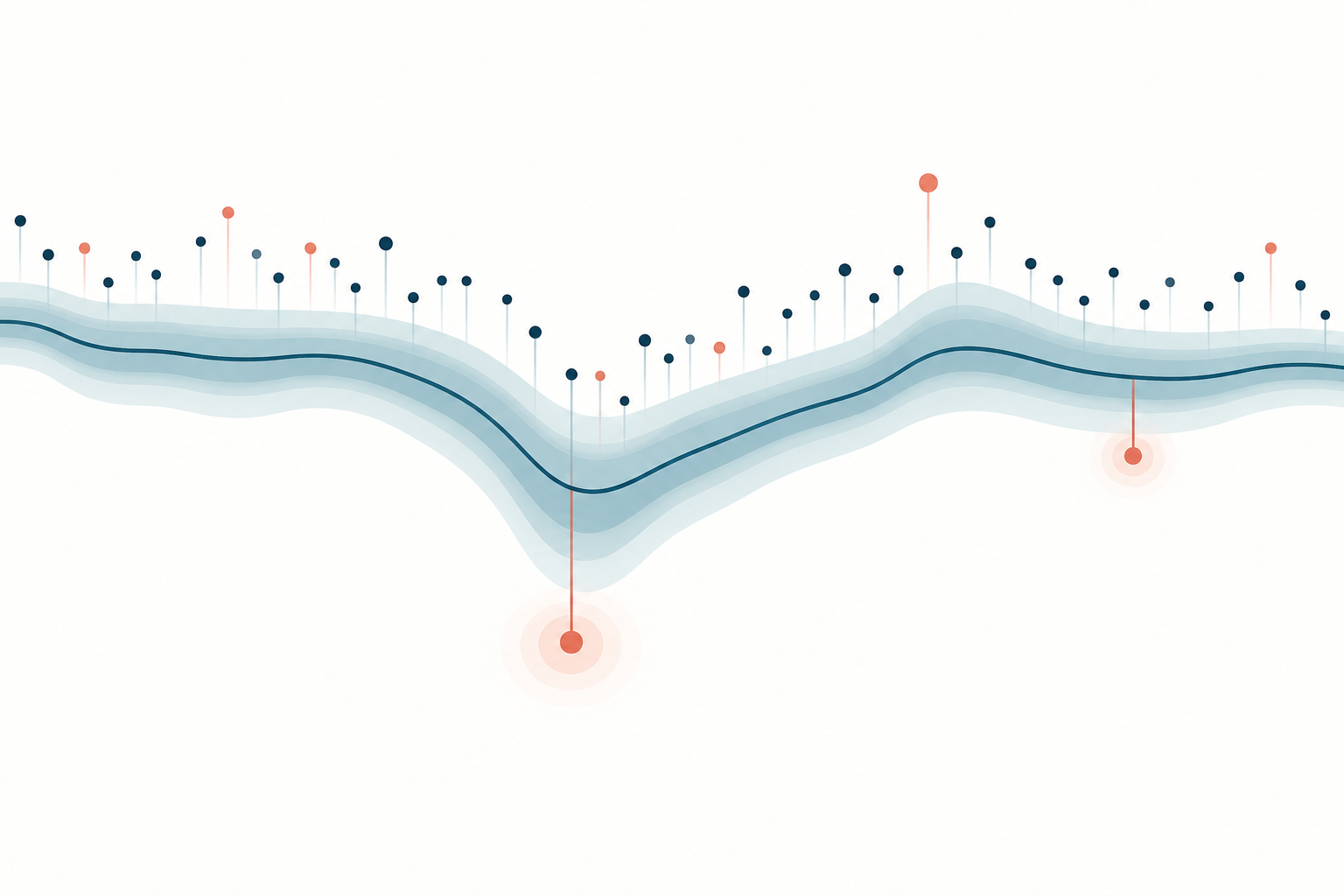
To let downside and upside observations affect the next loss quantile differently, define the positive and negative magnitudes \(L^+=\max(L,0)\) and \(L^-=\max(-L,0)\). One asymmetric-slope form is \[ v_t^\alpha=\beta_0+\beta_1v_{t-1}^\alpha+\beta_2L_{t-1}^{+}+\beta_3L_{t-1}^{-}. \] A positive portfolio loss enters through \(L^+\); a gain enters through \(L^-\). The two estimated slopes need not match. The sign convention changes if the model is written for returns and a lower-tail return quantile instead of positive losses, so a paper or implementation should state exactly what its dependent variable and “positive/negative part” mean.

This flexibility does not prove that markets have an asymmetric leverage effect. It lets the selected conditional quantile respond differently to the two branches, conditional on the chosen recursion and sample. Coefficients are estimated rather than known constants, and their signs and size depend on variable units and parameterization. Compare this form with a symmetric benchmark and evaluate both beyond their estimation sample.

<!-- Illustration placement: after section 3; text-free conceptual view of a conditional loss-quantile ribbon moving over time, responding more after a large loss than after an upside move, with a few conceptual threshold crossings. No axes, labels, values, or market data. -->

For candidate parameters \(\beta\), first generate the full recursive path \(v_t^\alpha(\beta)\). Then minimize the quantile, or check, loss: \[ \widehat\beta=\arg\min_\beta\sum_{t=1}^{T}\rho_\alpha\!\left(L_t-v_t^\alpha(\beta)\right), \qquad \rho_\alpha(u)=u\left(\alpha-\mathbf 1\{u<0\}\right). \] For an upper loss quantile, an underforecast has \(u>0\) and receives weight \(\alpha\); an overforecast has \(u<0\) and receives weight \(1-\alpha\). At \(\alpha=0.99\), the loss function makes a missed large loss costly relative to an equally sized excess buffer. It is not squared-error loss, and it does not choose coefficients to fit the conditional mean.

This is the regression-quantile idea developed by Koenker and Bassett (1978 paper), applied to a recursively generated quantile path. With linear quantile regression the objective has useful convex structure, but CAViaR's recursive nonlinear forms can make optimization sensitive to starting values and local minima. A practical fit should record the objective, parameter restrictions, optimization procedure, convergence checks, and alternative starts; standard least-squares output is not a substitute for quantile-regression inference.

The first recursive value \(v_0^\alpha\) must be supplied or estimated. One transparent choice is an empirical upper loss quantile from a presample window that ends before the evaluation period. Other implementations estimate an initial value jointly or use a documented burn-in. Whichever rule is chosen, apply it consistently across candidate forms and disclose how many observations initialize the recursion. If the lag coefficient is persistent, early initialization can influence many later forecasts.

Recursive quantile fits can be nonlinear in their parameters even when the displayed equation looks simple. Different starting vectors can converge to different local solutions; a converged optimizer only says it met its numerical stopping rule. Use multiple sensible starts where appropriate, inspect the resulting paths, and distinguish a numerical constraint—such as requiring a nonnegative loss threshold—from an economic fact. There is no single coefficient bound that guarantees stability for every CAViaR specification. Conditions depend on the form, identification, and behavior of the input process; the original paper's asymptotic results rely on explicit assumptions and exclude explosive cases.

Uncertainty also matters. Tail observations are sparse, especially at a 99% level, and the conditional density near the target quantile affects estimator precision. Parameter standard errors for nonlinear recursive quantiles need methods justified for that setting, such as suitable asymptotic estimators or a carefully designed bootstrap. Do not read a precise-looking fitted line as proof that tail risk is known precisely.

At origin \(t-1\), estimate parameters and generate \(v_t^\alpha\) using only returns and covariates available by that origin. Then compare the forecast with \(L_t\) after the period closes. If a model is re-estimated on a rolling or expanding window, every window must end at the stated forecast origin. Using \(L_t\) to form \(v_t^\alpha\), or using revised data that were unavailable at the time, leaks future information into the forecast.

Align the target with the actual portfolio and horizon. A daily VaR for a fixed-weight portfolio is not automatically a VaR for an account whose holdings change intraday, nor is a one-day quantile a multi-day risk forecast. Report return construction, currency, horizon, market close, portfolio rebalancing and the timing of each predictor. Predictor transformations, corporate actions, stale prices, and missing sessions can change the information set and the quantile dynamics.

The familiar recursion is naturally one-step ahead because \(v_t\) uses observed \(L_{t-1}\). For a multi-step forecast, later losses are not yet observed. Iterating the equation by inserting realized future losses would be look-ahead. A multi-period VaR needs an explicit procedure for the unknown future path—such as simulation or a separately specified multi-horizon model—and its assumptions should be evaluated separately.

Suppose a hypothetical 99% daily loss VaR follows the asymmetric-slope recursion above. Measure losses and \(v\) in percentage points, and choose illustrative—not estimated—parameters \(\beta_0=0.10\), \(\beta_1=0.80\), \(\beta_2=0.35\), and \(\beta_3=0.10\). If the prior forecast was \(2.00\%\) and yesterday's portfolio loss was \(3.00\%\), then \[ v_t^{0.99}=0.10+0.80(2.00)+0.35(3.00)+0.10(0)=2.75\%. \] The larger loss branch raises today's threshold in this example. If yesterday instead had a \(3.00\%\) gain, then \(L_{t-1}=-3.00\%\) and the other branch gives \[ v_t^{0.99}=0.10+0.80(2.00)+0.35(0)+0.10(3.00)=2.00\%. \] These coefficients are chosen only to demonstrate the recursion; another sample or parameterization can produce a different response.

If today's realized loss is \(3.20\%\), it exceeds the \(2.75\%\) forecast, so the hit indicator is one. A single hit does not establish that the model is poor, just as a day without a hit does not validate it. Under correct conditional calibration, the exception indicator should have conditional mean \(1-\alpha\) given forecast-origin information; over a long sample, its average should be near that rate, subject to sampling variation.

VaR is the risk quantity: a specified conditional loss quantile. CAViaR is one way to forecast that quantity. Expected Shortfall asks a different question: the average loss in the selected tail beyond VaR, under the relevant definition. A CAViaR quantile path alone does not determine that tail average or the shape of losses beyond the threshold. The guide to [VaR versus Expected Shortfall](/en/learn/value-at-risk-vs-expected-shortfall-explained) compares the measures.

GARCH models a conditional variance (or volatility) recursively; a distributional assumption for standardized innovations is then needed to translate variance into a VaR quantile. ARCH and GARCH are associated with Engle's ARCH model and Bollerslev's GARCH extension90063-1). CAViaR directly models the quantile and does not require a full conditional density, although it still makes assumptions through its chosen dynamics. The indirect-GARCH CAViaR specification is a special bridge between the two approaches, not evidence that all CAViaR models are GARCH. See the separate guide to [GARCH volatility clustering](/en/learn/volatility-clustering-garch-explained).

A low in-sample quantile loss is not an out-of-sample risk certificate. Reserve a chronological evaluation period, produce each forecast using only past information, and report both the hit rate and whether hits cluster or can be predicted from past information. An unconditional frequency test such as Kupiec's (1995) and a conditional coverage test such as Christoffersen's (1998) answer different questions; Engle and Manganelli's dynamic-quantile test examines selected restrictions on centered hits and chosen instruments. None of them tests every possible misspecification. For the mechanics of exception-sequence tests, see [VaR backtesting](/en/learn/value-at-risk-backtesting-kupiec-christoffersen-explained). To compare two quantile forecasts instead, score both with the same check loss on matched dates and compare the dependent loss differential using a [Diebold–Mariano test](/en/learn/diebold-mariano-test-forecast-accuracy-explained); that tests relative forecast loss, not VaR calibration or trading profit.

Results can change with the tail probability, recursion, initialization, estimation window, portfolio, and evaluation dates. A model that fits one quantile may fit another poorly, and independently estimated quantiles can cross. Structural breaks, clustered extremes, sparse tail data, changing holdings, market gaps, liquidity, and execution costs are not solved by a recursive VaR equation. VaR also says nothing about the severity of losses after an exception. Treat the result as a model-based risk threshold to monitor, not a loss cap, a forecast of profit, or a standalone trading rule.